Spatial interpolation on Earth as a 3D sphere

Spatial interpolation at Earth scale

Earth map is usually presented flat. Geographical coordinates usually go from -180° to +180°. Spatial interpolations using coordinates may be tricky as -180° is equal to +180°. Here I propose a way to realize spatial interpolations on Earth as a sphere and then map the outputs in 3D using rgl. The complete R-script extracted from this post is here on my github.

Random dataset

Let’s create a random dataset with observations of presences and absences over the globe (This is simulated with a little spatial auto-correlation North / South). We do not account for possible difference between terrestrial and oceans areas.
I use a ‘modulo’ trick to restrict coordinates between -180° and +180°. This is just for me to keep a trace of it (otherwise I could have used runif to simulate data).

# library(sp)
library(rgdal)
library(sf)
library(raster)
library(ggplot2)

# Simulate dataset with a little spatial auto-correlation
set.seed(42)
n <- 30
obs <- rbind(data.frame(lon = rnorm(n, 0, 180),
                      lat = rnorm(n, 50, 35),
                      value = 0),
           data.frame(lon = rnorm(n, 180, 180),
                      lat = rnorm(n, -50, 35),
                      value = 1))
# Modulo trick 
obs$lon <- obs$lon %% 360 -180
obs$lat <- obs$lat %% 180 -90

# Transform points as spatial points with sf ----
obs_sf <- st_as_sf(obs, coords = c("lon", "lat"),
                   crs = 4326)

# Plot on a worldmap
worldmap <- borders("world",
                    colour = "#fefefe",
                    fill = "#808080"
                    )

# Plot over a worldmap
ggplot() + worldmap +
  geom_point(data = obs,
             aes(x = lon, y = lat,
                 colour = factor(value))) +
  coord_quickmap()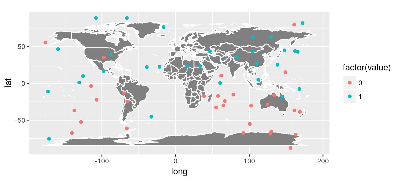

Inverse distance interpolation

A simple interpolation is the inverse distance interpolation. We can calculate distances between observations and world map using great circle.

• Create an empty raster that will be used as a target for interpolations.
• Transform points as spatial points with library sf
• Calculate (great circle) distances between points and raster cells
• Interpolate using inverse distance interpolation

# Create an empty world raster ----
ny <- 41
nx <- 80
r <- raster(
  nrows = ny, ncols = nx,
  crs = '+proj=longlat',
  xmn = -180, xmx = 180,
  ymn = -90, ymx = 90
)

# Transform raster as spatial points with sf
r_sf <- st_as_sf(as.data.frame(coordinates(r)),
                 coords = c("x", "y"),
                   crs = 4326)

# Distance between points and raster ----
obs.r.dists <- st_distance(obs_sf, r_sf)
obs.r.dists <- unclass(obs.r.dists)

# Inverse distance interpolation ----
## pred = 1/dist^idp
idp <- 2
inv.w <- (1/(obs.r.dists^idp))
z <- (t(inv.w) %*% matrix(obs$value)) / apply(inv.w, 2, sum)

# Fill in raster for predictions
r.pred <- r
values(r.pred) <- z

# Plot prediction raster
worldmap_predict <- borders("world",
                            colour = "#05050541",
                            fill = NA,
                            size = 0.5
)

rasterVis::gplot(r.pred) +
  geom_tile(aes(fill = value)) +
  scale_fill_gradient2(low = 'red', mid = "yellow",
                       high = 'green', midpoint = 0.5) +
  geom_point(data = obs,
             aes(x = lon, y = lat, colour = factor(value))) +
  worldmap_predict +
  guides(colour = FALSE) +
  coord_quickmap()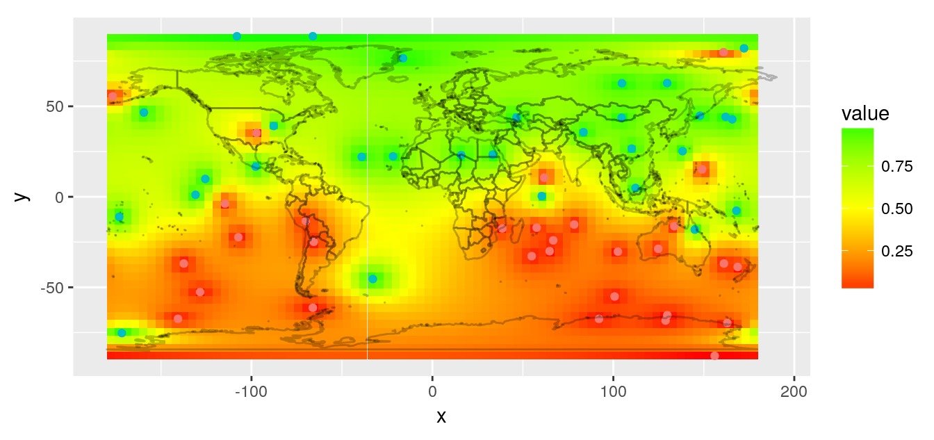

Kriging with user defined distances

To interpolate the dataset, you may want to use kriging. This interpolation relies on a variogram allowing to make use of the spatial structure of the data (contrary to idw which is fixed by the user).
For interpolations with custom distances and obstacles, I created the (totally in-development) GeoDist R-library. Here we do not have obstacles, but we have a user-defined distance matrix based on great circle distances that we want to use to fit a variogram and interpolate on the map. In GeoDist, I modified some functions of geoR so that it can fit a variogram and interpolate using a distance matrix defined by the user.

We calculate the variogram according to our own great circle distance matrix with GeoDist::variog.dist.

library(GeoDist)
# Transform data as geodata for geoR library
datageo <- as.geodata(obs, data.col = "value")
# Calculate distances between observations
obs.obs.dists <- st_distance(obs_sf)
obs.obs.dists <- unclass(obs.obs.dists)
# Create variogram with custom distances
data.v <- variog.dist(
  datageo, 
  trend = "cte",
  dist.mat = obs.obs.dists,
  max.dist = max(obs.obs.dists),
  breaks = seq(0, max(obs.obs.dists), length.out = 10))
# Fit variogram
data.vfit <- geoR::variofit(
  data.v, 
  cov.model = "exponential")
# Plot
plot(data.v); lines(data.vfit, col = "blue")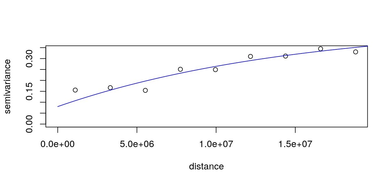

We use the variogram to predict on the entire map, also using custom distances with GeoDist::krige.conv.dist.

# Distances to raster
obs.r.dists <- st_distance(obs_sf, r_sf)
obs.r.dists <- unclass(obs.r.dists)
# Distances between raster locations
r.r.dists <- st_distance(r_sf, r_sf)
r.r.dists <- unclass(r.r.dists)
# Krige with custom distances
r.krige <- krige.conv.dist(
  geodata = datageo, 
  locations = coordinates(r),
  krige = krige.control(obj.model = data.vfit),
  dist.mat = obs.obs.dists,
  loc.dist = obs.r.dists,
  loc.loc.dist = r.r.dists)
# Fill in raster with predictions
r.pred <- r
values(r.pred) <- r.krige$predict
# Plot prediction raster
rasterVis::gplot(r.pred) +
  geom_tile(aes(fill = value)) +
  scale_fill_gradient2(low = 'red', mid = "yellow",
                       high = 'green', midpoint = 0.5) +
  geom_point(data = obs,
             aes(x = lon, y = lat, colour = factor(value))) +
  worldmap_predict +
  guides(colour = FALSE) +
  coord_quickmap()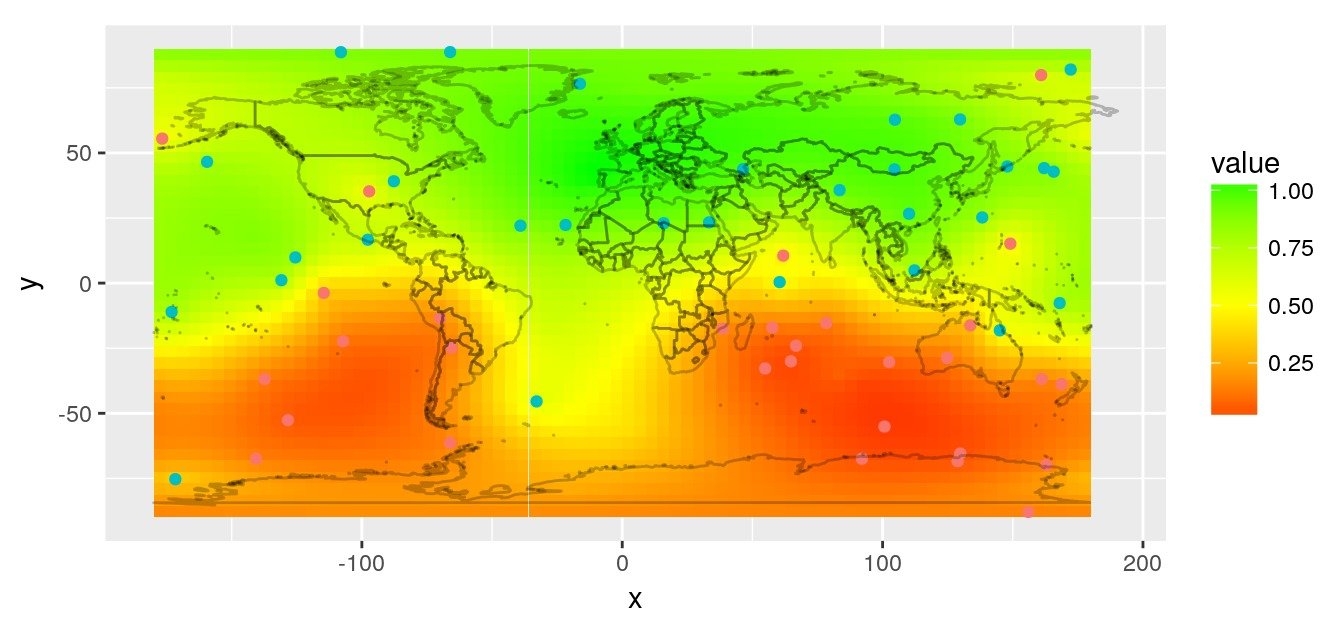

Fit a gam model on 3D-coordinates

If you want to model the global distribution, with a GAM for instance, using latitude and longitude, you will face the discontinuity in the longitude coordinates. In that case, it may be preferable to use 3D-cartesian coordinates of the globe. In GeoDist, I included the function sph2car to transform geographical coordinates into cartesian. This is a modification of sphereplot::sph2car, which allows to include the ellipsoid flattening (geosphere::refEllipsoids()).

# Transform data in 3D ----
library(ggplot2)
library(maptools)
library(raster)
library(rgl)

# Transform observation in cartesian coords
obs.cart <- data.frame(sph2car(obs[,1:2]), value = obs$value)
# Approximation with a gam model
library(mgcv)
gam1 <- gam(value ~ te(x, y, z, k = 3),
            data = obs.cart,
            family = binomial)
# Predict on Raster
r.cart <- data.frame(sph2car(coordinates(r)))
pred <- predict(gam1, r.cart, type = "response")
r.pred <- r
values(r.pred) <- c(pred)

# Plot prediction raster
rasterVis::gplot(r.pred) +
  geom_tile(aes(fill = value)) +
  scale_fill_gradient2(low = 'red', mid = "yellow",
                       high = 'green', midpoint = 0.5) +
  geom_point(data = obs,
             aes(x = lon, y = lat, colour = factor(value))) +
  worldmap_predict +
  guides(colour = FALSE) +
  coord_quickmap()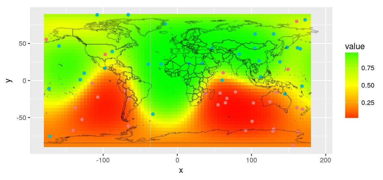

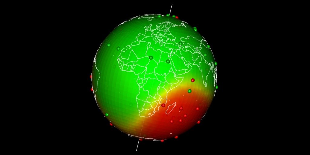
Plot predictions on a globe with rgl

There are different ways to get a projection allowing to show Earth as a globe and to create rotation gif. In my case, I like using rgl library because the output in interactive and I can easily travel the world with the mouse.

Projection of our predicted map within a rgl 3D plot requires a few steps:

• Build the 3D representation of the prediction raster with triangulation
  • [Edit: 2017-11-06] Directly create 3D triangulation using geometry::convhulln (Thanks to @mdsumner)
  • [removed] Triangulate both halves of the globe separately using library deldir
  • [removed] Combine both halves
• Create color for each triangle facet according to predictions
• Draw the 3D rgl map
  • Drape the globe with predictions using triangles3d
  • Add observations as spheres3d
  • Add Earth rotation axis for fun
• Add a map of the world on the 3d sphere
  • Retrieve geographical coordinates and transform as cartesian with function sph2car
• Use transform3d and rotationMatrix functions to rotate Earth and take snapshots
  • Create a gif

# Plot in 3d using rgl ----
library(geometry)
library(dplyr)
library(rgl)

# ---- Edit - 2017-11-06 ----
# Triangulate entire globe directly with geometry ----
# Thanks to Michael Sumner @mdsumner
tri3d <- geometry::convhulln(r.cart)
r.cart.tri <- r.cart[t(tri3d), ] %>%
  mutate(n = c(t(tri3d)))

# Edit: Kept here as reminder but simpler with "geometry"
if (FALSE) {
  # _With deldir = 2D triangulation ----
  library(deldir)
  # Triangulate top half of the globe
  r.cart.top <- as.data.frame(r.cart) %>% as.tbl() %>%
    mutate(n = 1:n()) %>%
    filter(z >= 0)
  r.cart.top.del <- deldir(as.data.frame(r.cart.top[,1:2]))
  r.cart.top.tri <- do.call(rbind, triang.list(r.cart.top.del))
  r.cart.top.tri$n <- r.cart.top$n[r.cart.top.tri$ptNum]
  
  # Triangulate bottom half of the globe
  r.cart.bottom <- as.data.frame(r.cart) %>% as.tbl() %>%
    mutate(n = 1:n()) %>%
    filter(z <= 0)
  r.cart.bottom.del <- deldir(as.data.frame(r.cart.bottom[,1:2]))
  r.cart.bottom.tri <- do.call(rbind, triang.list(r.cart.bottom.del))
  r.cart.bottom.tri$n <- r.cart.bottom$n[r.cart.bottom.tri$ptNum]
  
  # Combine top and bottom
  r.cart.tri <- rbind(r.cart.top.tri, r.cart.bottom.tri) %>%
    mutate(z = r.cart[.$n,"z"])
}
# ---- End of Edit ----

# Define a vector of colors for predictions
n.break <- 20
colors <- alpha(colorRampPalette(c("red", "yellow", "green"))(n.break), .4)
brk <- seq(0, 1, len = n.break + 1)
pred.col <- colors[as.numeric(as.character(
  cut(pred, breaks = brk, include.lowest = TRUE, labels = 1:n.break)))]

# Print in 3d
triangles3d(r.cart.tri$x,
            r.cart.tri$y,
            r.cart.tri$z,
            col = pred.col[r.cart.tri$n],
            alpha = 0.9,
            specular = "black")
# Observation with radius in scale of coordinates
spheres3d(obs.cart[,1:3],
          radius = rep(0.2e6, nrow(obs.cart)),
          color = obs.cart[,4] + 2)
# Black background
rgl.bg(color = c("black"))
# Add Earth rotation axe
segments3d(x = c(0,0),
           y = c(0,0),
           z = c(min(r.cart.tri$z)*1.2, 
                 max(r.cart.tri$z)*1.2),
           col = "white",
           lwd = 2)

# Map world on the 3d sphere ----
library(rworldmap)
data(countriesCoarse)

for (i in 1:nrow(countriesCoarse)) { # i <- 1
  Pols <- countriesCoarse@polygons[[i]]  
  for (j in 1:length(Pols)) { # j <- 1
    lines3d(data.frame(sph2car(
      countriesCoarse@polygons[[i]]@Polygons[[j]]@coords
    )), col = "white", lwd = 2)
  }
}

# Rotate and save as gif
# extraWD: directory where to save img of rotation
nb.img <- 45
angle.rad <- seq(0, 2*pi, length.out = nb.img)
# NorthPole on top, Europe-Africa in front.
uM0 <- rotationMatrix(-pi/2, 1, 0, 0) %>%
  transform3d(rotationMatrix(-2, 0, 0, 1)) %>%
  transform3d(rotationMatrix(-pi/12, 1, 0, 0))
# Change viewpoint
rgl.viewpoint(theta = 0, phi = 0, fov = 0, zoom = 0.7,
              userMatrix = uM0)

for (i in 1:nb.img) {
  # Calculate matrix rotation
  uMi <- transform3d(uM0, rotationMatrix(-angle.rad[i], 0, 0, 1))
  # Change viewpoint
  rgl.viewpoint(theta = 0, phi = 0, fov = 0, zoom = 0.7,
                userMatrix = uMi)
  # Save image
  filename <- paste0(extraWD, "/gif/pic", formatC(i, digits = 1, flag = "0"), ".png")
  rgl.snapshot(filename)    
}
# Create gif
system(glue::glue("convert -delay 10 {extraWD}/gif/*.png -loop 0 ../../static{StaticImgWD}/Globe3D_rgl.gif"))

The complete R-script extracted from this post is here on my github.