Polygons tint band with leaflet and simple feature (library sf)

Add a tint band (aka shapeburst fill) in leaflet

Stackoverflow is again a source of inspiration. I found this question on tint bands in leaflet, not related to R originally but I though I could answer it with R easily. This is also a good one for me to play with this new simple feature library sf and use it with leaflet. My simple solution is to create a new multipolygon from the original one, but with holes inside, so that we only get a doughnut polygon for each area. As raised by my question on stackoverflow (again…), I recently remarked that it could be tricky to plot multipolygons with holes in ggplot2 with SpatialPolygons from library sp, which is another reason to use library sf.

Get French regions data

Let’s use some French regions polygons and attribute one colour to each region. I like piratepal colours of library yarrr.

fra.sp <- getData('GADM', country = 'FRA', level = 1, path = extraWD)
fra.sf <- st_as_sf(fra.sp)

ggplot(fra.sf) +
  geom_sf(aes(fill = NAME_1), alpha = 0.8) +
  scale_fill_manual(values = rep(unique(yarrr::piratepal("basel")),
                                 length.out = nrow(fra.sf))) +
  guides(fill = FALSE)

Figure 1: French regions colored using rstat and library sf

Create future holes with buffer

We create the future holes with a smaller buffer area. Here, st_buffer returns an object without geometry type (geometry type: GEOMETRY), which prevents it to be plot (Error in CPL_gdal_dimension(st_geometry(x), NA_if_empty)). A workaround is to use st_cast after.

fra.sf.buf <- st_cast(st_buffer(fra.sf, dist = -0.1))

ggplot() +
  geom_sf(data = fra.sf.buf, aes(fill = factor(NAME_1)), alpha = 0.8) +
  geom_sf(data = fra.sf,
          colour = "grey20", fill = "transparent",
          size = 0.5) +
  scale_fill_manual(values = rep(unique(yarrr::piratepal("basel")),
                                 length.out = nrow(fra.sf))) +
  guides(fill = FALSE)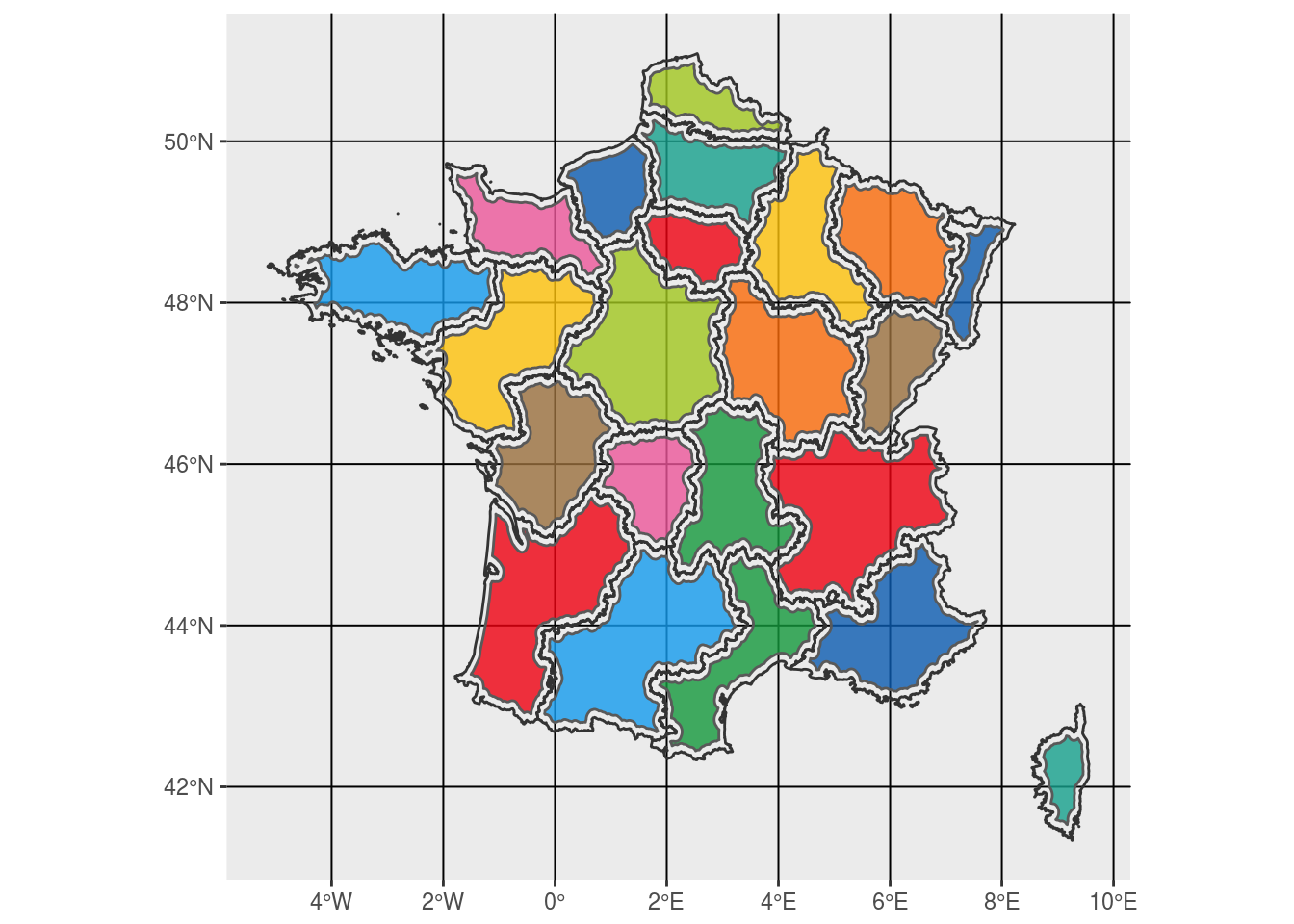

Figure 2: Polygon holes of future tint bands

Create holes in the original polygons

To create the doughnuts using original and buffer polygons, I used st_difference. However as discussed with edzer in the sf github repository, I had to transform the buffer polygons into a Multipolygon of a unique Multipolygon using st_combine. Moreover, because the resulting Multipolygon object as no identified geometry, I had to pass it through st_cast.

# st_difference work if the mask is a unique multipolygon
fra.sf.buf.comb <- fra.sf.buf %>% st_combine() %>% st_sf()
fra.sf.doug <- st_difference(fra.sf, fra.sf.buf.comb) %>% st_cast()

ggplot() +
  geom_sf(data = fra.sf.doug, aes(fill = factor(NAME_1)),
          alpha = 0.6, colour = "transparent") +
  # geom_sf(data = fra.sf, colour = "grey20") +
  scale_fill_manual(values = rep(unique(yarrr::piratepal("basel")),
                                 length.out = nrow(fra.sf.doug))) +
  guides(fill = FALSE)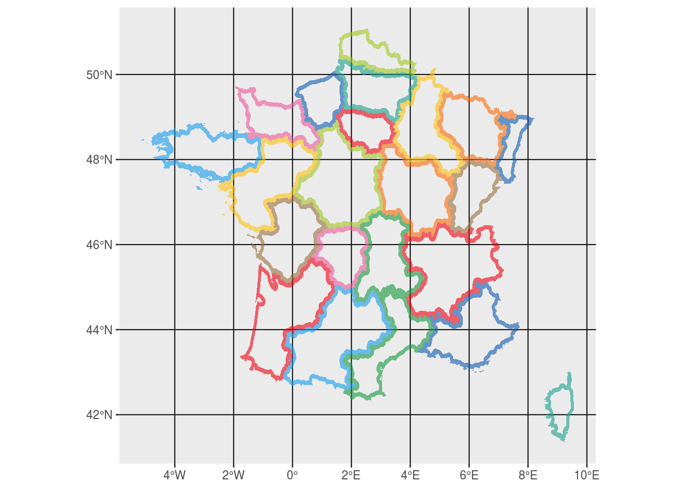

Figure 3: Doughnuts style tint bands

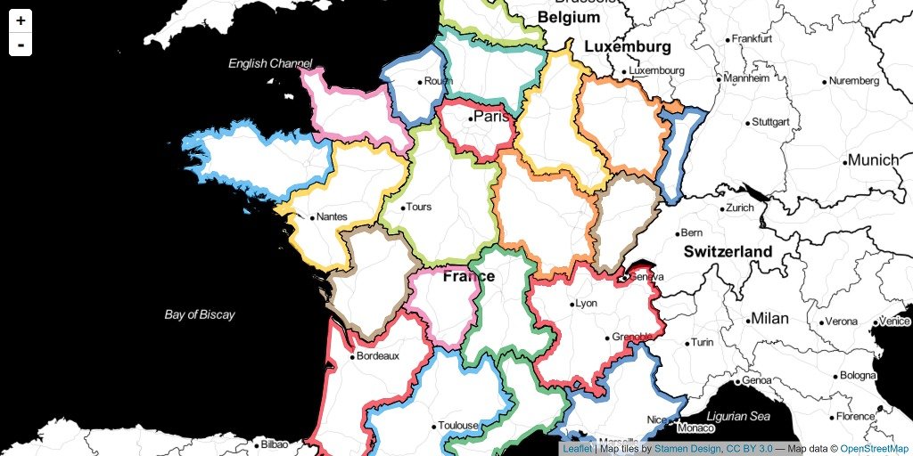
Output tint bands in leaflet

To allow for a quick view, polygons were simplified with st_simplify. You’ll see it if you zoom.

# Simplify geometry to get a lighter widget
# Separate "Rhône-Alpes", "Franche-Comté", "Bourgogne", "Bretagne" as it does not support to much simplification
fra.sf.doug.simple1 <- st_simplify(filter(fra.sf.doug, NAME_1 %in% c("Rhône-Alpes", "Franche-Comté")), dTolerance = 1e-4)
fra.sf.doug.simple2 <- st_simplify(filter(fra.sf.doug, NAME_1 %in% c("Bourgogne")), dTolerance = 1e-5)
fra.sf.doug.simple3 <- st_simplify(filter(fra.sf.doug, NAME_1 %in% c("Bretagne")), dTolerance = 1e-2)
fra.sf.doug.simple4 <- st_simplify(filter(fra.sf.doug, !NAME_1 %in% c("Rhône-Alpes", "Franche-Comté", "Bourgogne", "Bretagne")), dTolerance = 0.02)
fra.sf.doug.simple <- rbind(fra.sf.doug.simple1, fra.sf.doug.simple2, fra.sf.doug.simple3,  fra.sf.doug.simple4) %>% st_cast()
fra.sf.simple <- st_simplify(fra.sf, dTolerance = 0.02)

Now we can use it to produce a leaflet map with tinted bands having transparency and original polygons in black.

factpal <- colorFactor(rep(unique(yarrr::piratepal("basel")),
                                 length.out = nrow(fra.sf.doug.simple)),
                       fra.sf.doug.simple$NAME_1)

# leaflet widget
m <- leaflet() %>%
  addProviderTiles(providers$Stamen.Toner) %>%
  addPolygons(data = fra.sf.doug.simple, weight = 1, smoothFactor = 0.75,
    opacity = 0, fillOpacity = 0.6,
    color = "#000000",
    fillColor = ~factpal(fra.sf.doug.simple$NAME_1),
    highlightOptions = highlightOptions(color = "white", weight = 2,
      bringToFront = TRUE)) %>%
  addPolygons(data = fra.sf.simple, weight = 1, smoothFactor = 0.75,
    opacity = 1.0, fillOpacity = 0,
    color = "#000000")

The full rmarkdown script

If you want to reproduce these figures, the full rmarkdown script is available here on my github.