The #30DayMapChallenge was initiated by Topi Tjukanov on Twitter. This is open to anyone who would like to show a map, whatever the software is. In this blog post, I will show maps made with R. I add constraints to myself for fun. This week, I will use {ggplot2} to create maps.
Packages
library(dplyr)
library(sf)
library(raster)
library(ggplot2)
library(readr)
library(tmap)
# library(hexbin)

## Customize
# Test for font family
# extrafont::font_import(prompt = FALSE)
font <- extrafont::choose_font(c("Nanum Pen", "Lato", "sans"))

my_blue <- "#1e73be"
my_theme <- function(font = "Nanum Pen", ...) {
  theme_dark() %+replace%
    theme(
      plot.title = element_text(family = font,
                                colour = my_blue, size = 18),
      plot.subtitle = element_text(family = font, size = 15),
      # text = element_text(size = 13), #family = font,
      plot.margin = margin(4, 4, 4, 4),
      plot.background = element_rect(fill = "#f5f5f2", color = NA),
      legend.text = element_text(family = font, size = 10),
      legend.title = element_text(family = font),
      # legend.text = element_text(size = 8),
      legend.background = element_rect(fill = "#f5f5f2"),
      ...
    )
}
Data
Loire-atlantique in France
# extraWD <- "." # Uncomment for the script to work
# Read shapefile "Departement.shp"
France_L93 <- st_read(file.path(extraWD, "DEPARTEMENT.shp"), quiet = TRUE)
LoireATl_L93 <- st_read(file.path(extraWD, "Intersect_ZE_L93.shp"), quiet = TRUE)

# Create polygon for oceanic area (difference with terrestrial)
LoireATl_ocean_L93 <- st_bbox(LoireATl_L93) %>%
  st_as_sfc()  %>%
  st_difference(st_union(LoireATl_L93))

ggplot(LoireATl_ocean_L93) +
  geom_sf(fill = my_blue) +
  labs(
    title = "bbox difference with terrestrial"
  ) +
  theme_dark()

# Read trafic in Loire-atlantique 2010, 2013
trafic_L93 <- st_read(file.path(extraWD, "trafic_L93.shp"), quiet = TRUE)

# Trafic merged with roads
RoadsMergeTrafic_Dpt44_L93 <- st_read(
  file.path(extraWD, "RoadsMergeTrafic_Dpt44_L93.shp"),
  quiet = TRUE) %>%
  st_line_merge()
Points: Spatial points and facets with {ggplot2}
ggplot() +
  geom_sf(data = LoireATl_ocean_L93, colour = NA, fill = my_blue, alpha = 0.75) +
  geom_sf(data = LoireATl_L93, colour = "grey80", fill = NA) +
  geom_sf(data = trafic_L93, aes(size = TV),
          colour = "white", alpha = 0.5,
          inherit.aes = FALSE, show.legend = "point") +
  facet_wrap(~ANNEE_REF) +
  coord_sf(crs = st_crs(trafic_L93),
           xlim = c(st_bbox(trafic_L93)$xmin, st_bbox(trafic_L93)$xmax),
           ylim = c(st_bbox(trafic_L93)$ymin, st_bbox(trafic_L93)$ymax)) +
  scale_colour_gradientn(
    "Nombre",
    colours = RColorBrewer::brewer.pal(9, "YlOrRd"),
    trans = "log",
    breaks = c(400, 1000, 3000, 8000, 22000)
    ) +
  scale_size(range = c(0.25, 4)) +
  # guides(size = FALSE) +
  labs(x = "", y = "",
       title = "Trafic sur les routes de Loire-atlantique",
       subtitle = "Nombre de voitures (moyenne journalière au point de contrôle)",
       caption = "@statnmap; Source: data.loire-atlantique.fr",
       size = "Nombre\nvéhicules") +
  theme_dark(base_size = 10) +
  theme(plot.title = element_text(colour = my_blue))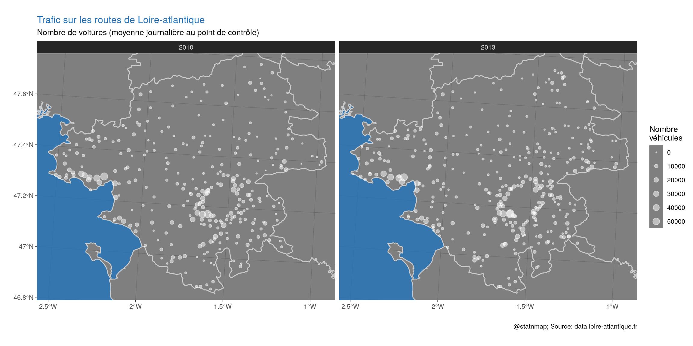
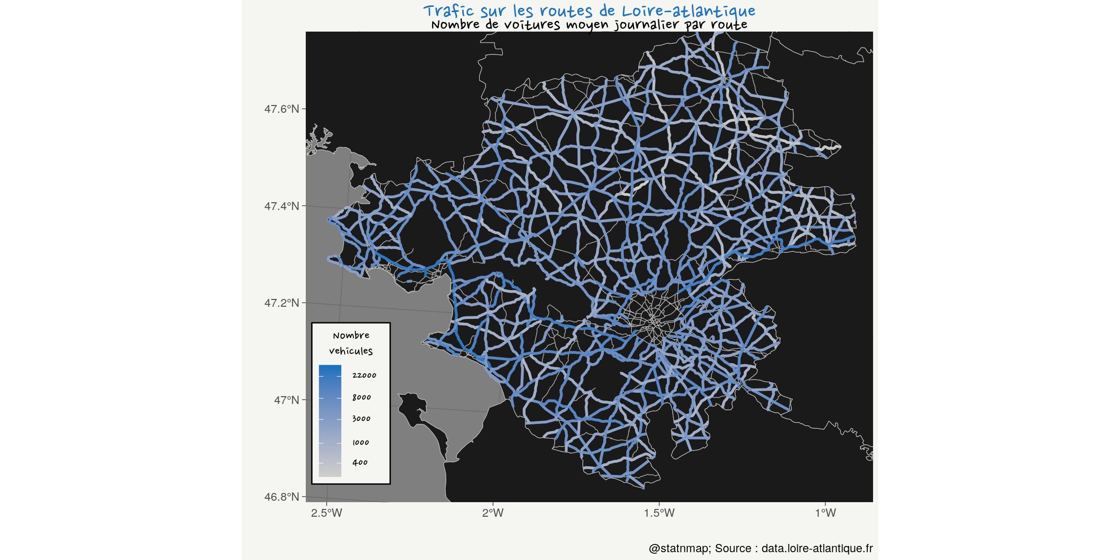
Lines: Color spatial lines according to numeric variable in {ggplot2}
# Figure
ggplot() +
  geom_sf(data = LoireATl_L93, colour = "grey80", fill = "grey10", size = 0.2) +
  geom_sf(data = RoadsMergeTrafic_Dpt44_L93, colour = "grey70", size = 0.25) +
  geom_sf(data = filter(RoadsMergeTrafic_Dpt44_L93, !is.na(TV)),
          aes(colour = TV),
          # aes(alpha = -TV, size = TV), # No alpha with lines
          size = 1,
          show.legend = "line", inherit.aes = FALSE) +
  coord_sf(crs = st_crs(trafic_L93)) +
  xlim(st_bbox(trafic_L93)$xmin, st_bbox(trafic_L93)$xmax) +
  ylim(st_bbox(trafic_L93)$ymin, st_bbox(trafic_L93)$ymax) +
  scale_colour_gradient(
    low = "grey80",
    high = my_blue,
    trans = "log", breaks = c(400, 1000, 3000, 8000, 22000)
  ) +
  labs(x = "", y = "",
       title = "Trafic sur les routes de Loire-atlantique",
       subtitle = "Nombre de voitures moyen journalier par route",
       caption = "@statnmap; Source : data.loire-atlantique.fr",
       colour = "Nombre\nvehicules"
  ) +
  my_theme(
    legend.position = c(0.08, 0.21)
  )
Polygons: Polygons unions and inside buffer areas
Polygons in polygons.
Inspired by my blog post on Polygons tint band with leaflet and simple feature (library sf)
# France union
France_union_L93 <- st_union(France_L93)
# _Negative buffer on France
France_dough <- st_buffer(France_union_L93, dist = -15000) %>%
  st_difference(France_union_L93, .)

# Pays de la loire union
PaysLoire_union_L93 <- France_L93 %>%
  filter(NOM_REG == "PAYS DE LA LOIRE") %>%
  st_union()
# _Negative buffer on PdL
PdL_dough <- st_buffer(PaysLoire_union_L93, dist = -10000) %>%
  st_difference(PaysLoire_union_L93, .)

# Loire-atlantique
LoireATl_small_L93 <- filter(LoireATl_L93, NOM_DEPT == "LOIRE-ATLANTIQUE")
# Negative buffer 1 on LA
LoireATl_dough1 <- st_buffer(LoireATl_small_L93, dist = -5000) %>%
  st_difference(LoireATl_small_L93, .)
# Negative buffer 2 on LA
LoireATl_dough2 <- st_buffer(LoireATl_small_L93, dist = -15000) %>%
  st_difference(st_buffer(LoireATl_small_L93, dist = -10000), .)
# Negative buffer 3 on LA
LoireATl_dough3 <- st_buffer(LoireATl_small_L93, dist = -25000) %>%
  st_difference(st_buffer(LoireATl_small_L93, dist = -20000), .)

# Plot
ggplot() +
  # France
  geom_sf(data = France_union_L93, fill = "grey50", colour = "grey20", size = 2) +
  geom_sf(data = France_dough, fill = my_blue, colour = NA) +
  # PdL
  geom_sf(data = PaysLoire_union_L93, fill = "grey70", colour = "grey20", size = 1.5) +
  geom_sf(data = PdL_dough, fill = my_blue, colour = NA) +
  # LA
  geom_sf(data = LoireATl_small_L93, fill = "grey90", colour = "grey20", size = 1) +
  geom_sf(data = LoireATl_dough1, fill = my_blue, colour = NA) +
  geom_sf(data = LoireATl_dough2, fill = my_blue, colour = NA) +
  geom_sf(data = LoireATl_dough3, fill = my_blue, colour = NA) +
  labs(
    title = "Loire-atlantique department...",
    subtitle = "...in Pays de la Loire region, in France",
    caption = "@statnmap; Source : ign.fr"
  ) +
  my_theme()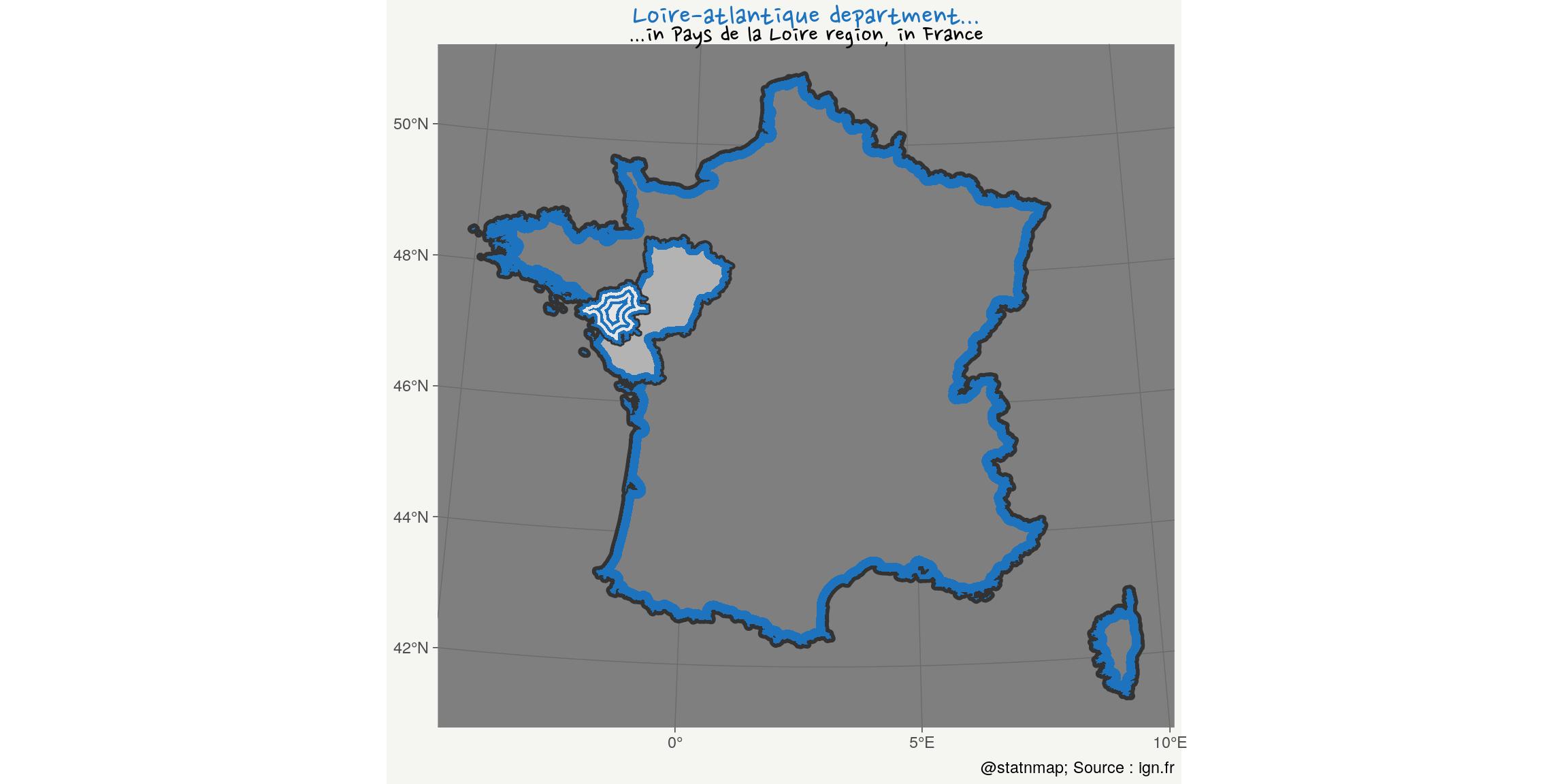
Hexagons: Draw hexagons and transform as spatial polygons
France is called “The Hexagon”. Let’s show why !
# France in hex
fr_bbox <- st_bbox(France_L93 %>% filter(!grepl("CORSE", NOM_DEPT)))
fr_hex <- hexbin::hexcoords(
  dx = (fr_bbox$xmax - fr_bbox$xmin)/2 + 15000
) %>%
  as_tibble() %>%
  bind_rows(.[1,]) %>%
  mutate(
    id = 1:n(),
    x = x + fr_bbox$xmin + 0.5 * (fr_bbox$xmax - fr_bbox$xmin) + 20000,
    y = y + fr_bbox$ymin + 0.5 * (fr_bbox$ymax - fr_bbox$ymin) - 30000
  ) %>%
  st_as_sf(coords = c("x", "y"), crs = 2154) %>%
  st_combine() %>%
  st_cast("POLYGON")

# Corse in hex
c_bbox <- st_bbox(France_L93 %>% filter(grepl("CORSE", NOM_DEPT)))
c_hex <- hexbin::hexcoords(
  dx = (c_bbox$xmax - c_bbox$xmin)/2 + 20000,
  dy = (c_bbox$ymax - c_bbox$ymin)/3
) %>%
  as_tibble() %>%
  bind_rows(.[1,]) %>%
  mutate(
    id = 1:n(),
    x = x + c_bbox$xmin + 0.5 * (c_bbox$xmax - c_bbox$xmin),
    y = y + c_bbox$ymin + 0.5 * (c_bbox$ymax - c_bbox$ymin)
    ) %>%
  st_as_sf(coords = c("x", "y"), crs = 2154) %>%
  st_combine() %>%
  st_cast("POLYGON")

ggplot() +
  geom_sf(data = fr_hex, fill = NA, colour = my_blue, size = 2) +
    geom_sf(data = c_hex, fill = NA, colour = my_blue, size = 2) +
  geom_sf(data = France_union_L93, fill = "grey60",
          colour = "grey20", size = 1) +
    labs(
      title = "France = L'Hexagone (regulier)",
      subtitle = "La Corse aussi (presque)...",
      caption = "@statnmap; Source : ign.fr"
    ) +
  my_theme()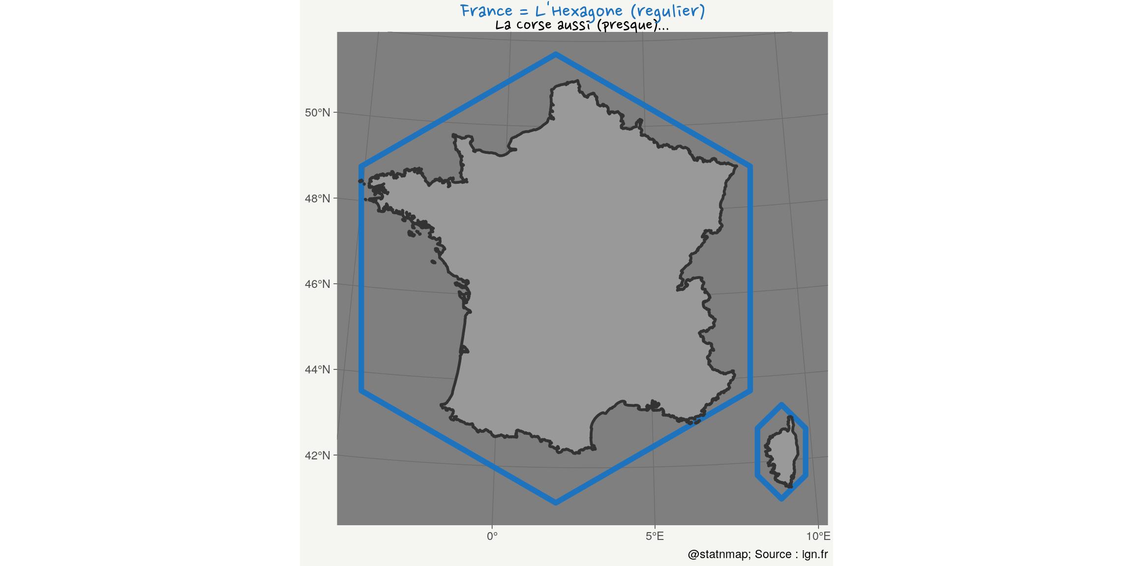
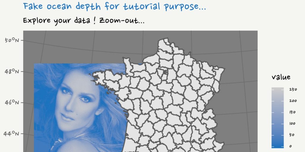
Raster: Images are rasters and can be added on maps
Images are rasters. If you are not convinced, you can look at articles in my “geohacking” category. You can also have a look at my SatRday Paris 2019 presentation: 2019-02 - Everything but maps with spatial tools - SatRday Paris (EN).
One day, I gave a tutorials on QGIS for master students at the University. They observed a specific study area. I asked to load a bathymetric raster file so that they could extract depth at sampling positions.
Because the project was already zoomed on the area, they did not remark that the raster file was indeed a picture of Céline Dion.
The objective was to tell them they had to explore their data and be sure about what they manipulate before using it for any analysis. I hope they got the message…
How can I reproduce this using R?
# image: 1125*1500
xmin <- -300000; xmax <- 800000; ymin <- 6100000
r <- raster::raster(file.path(extraWD, "celine-dion.jpeg"),
                    crs = st_crs(France_L93)$proj4string)
extent(r) <- c(xmin, xmax, ymin,  ymin + ((xmax-xmin)*1125/1500))

ext <- c(xmin = 250000, xmax = 500000, ymin = 6400000, ymax = 6800000)
cropping_area <-  st_bbox(ext) %>% st_as_sfc()
r_cropped <- raster::crop(r, extent(ext))
France_cropped <- France_L93 %>% st_crop(cropping_area)

rasterVis::gplot(r_cropped, maxpixels = 750000) +
  geom_tile(aes(fill = value)) +
  geom_sf(data = France_cropped, inherit.aes = FALSE) +
  scale_fill_gradient(
    low = my_blue,
    high = "grey80"
  ) +
  labs(
    title = "Fake ocean depth for tutorial purpose...",
    subtitle = "Explore your data !",
    caption = "@statnmap",
    x = NULL, y = NULL
  ) +
  coord_sf(expand = FALSE) +
  my_theme()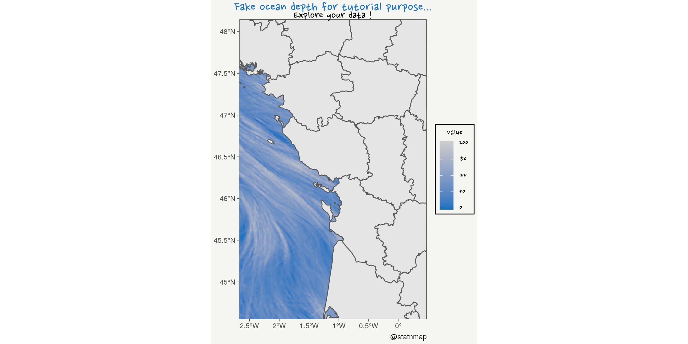
Zoom-out !
rasterVis::gplot(r, 100000) +
  geom_tile(aes(fill = value)) +
  geom_sf(data = France_L93, inherit.aes = FALSE) +
  scale_fill_gradient(
    low = my_blue,
    high = "grey80"#,
    # trans = "log", breaks = c(400, 1000, 3000, 8000, 22000)
  ) +
  labs(
    title = "Fake ocean depth for tutorial purpose...",
    subtitle = "Explore your data ! Zoom-out...",
    caption = "@statnmap",
    x = NULL, y = NULL
  ) +
  my_theme()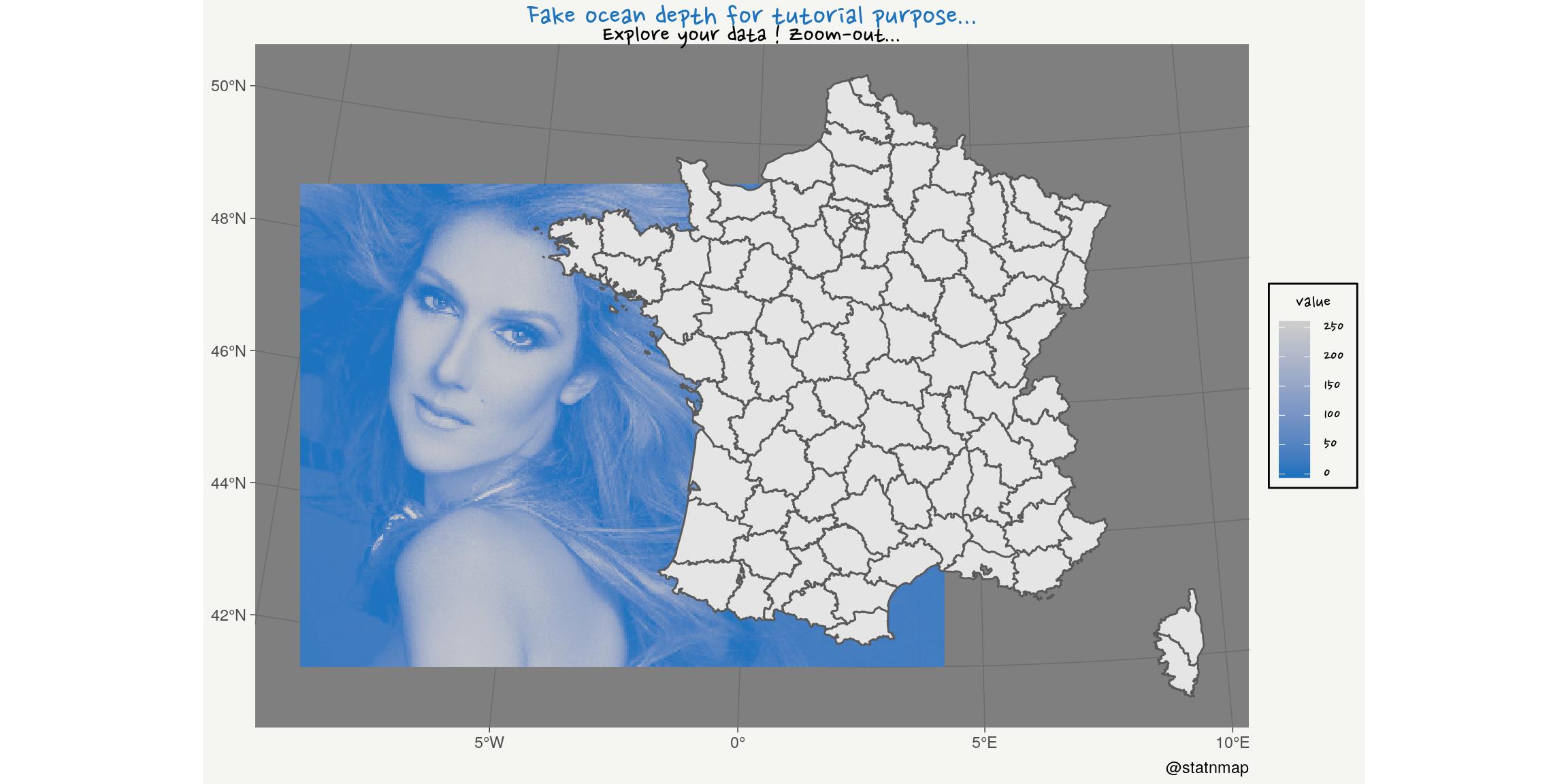
Blue: Map of fish species probability of presence and inset using {ggplot2}
To me, originally a marine biologist, blue is for the ocean. Let’s sea if I can retrieve predictions of juvenile common sole distribution from my phD…
Rochette, S., Rivot, E., Morin, J., Mackinson, S., Riou, P., Le Pape, O. (2010). Effect of nursery habitat degradation on flatfish population renewal. Application to Solea solea in the Eastern Channel (Western Europe). Journal of sea Research, Volume 64, p34-44. doi: 10.1016/j.seares.2009.08.003 , Open Access version : http://archimer.ifremer.fr/doc/00008/11921/.
# World map
countries <- rnaturalearth::ne_countries(returnclass = "sf", scale = "large")
# Europe
Europe <- countries %>%
  filter(continent == "Europe")
# Proba presence solea
solea <- raster(file.path(extraWD,
                          "Raster_PresenceProbability_Predictions.tif"))

# Projet raster to L93
solea_l93 <- projectRaster(
  solea,
  crs = st_crs(France_L93)$proj4string)

# Window
g_window <- ggplot() +
  geom_sf(data = Europe, fill = "white") +
  geom_sf(data = st_bbox(solea_l93) %>% st_as_sfc(),
          colour = my_blue, fill = NA, size = 2) +
  coord_sf(xlim = c(-10, 20), ylim = c(40, 60),
           expand = FALSE) +
  theme_bw() +
  theme(
    panel.background = element_rect(
      fill = scales::alpha(my_blue, 0.5)),
    axis.text = element_blank(),
    axis.ticks = element_blank()
    )

# Solea img
img_solea <- magick::image_read(file.path(extraWD, "Solea.gif"))
g_solea <- magick::image_ggplot(img_solea)

# Plot
rasterVis::gplot(solea_l93, maxpixels = 1623075) +
  geom_tile(aes(fill = value)) +
  geom_sf(data = Europe, inherit.aes = FALSE,
          size = 0.1, fill = "white") +
  scale_fill_gradient(
    high = my_blue,
    low = "grey80", na.value = NA,
    limits = c(0, NA)
  ) +
  labs(
    title = "Probability of presence of Young-of-the-year common sole",
    subtitle = "Eastern Channel",
    caption = "@statnmap",
    x = NULL, y = NULL,
    fill = "Probability"
  ) +
  coord_sf(crs = 2154,
             xlim = bbox(solea_l93)[1,],
           ylim = bbox(solea_l93)[2,]) +
  my_theme() +
  annotation_custom(grob = ggplotGrob(g_window),
    xmin = 540000, xmax = 630000,
    ymin = 6882000, ymax = 6982000) +
  annotation_custom(grob = ggplotGrob(g_solea),
    xmin = 331500, xmax = 430000,
    ymin = 6982000, ymax = 7052000)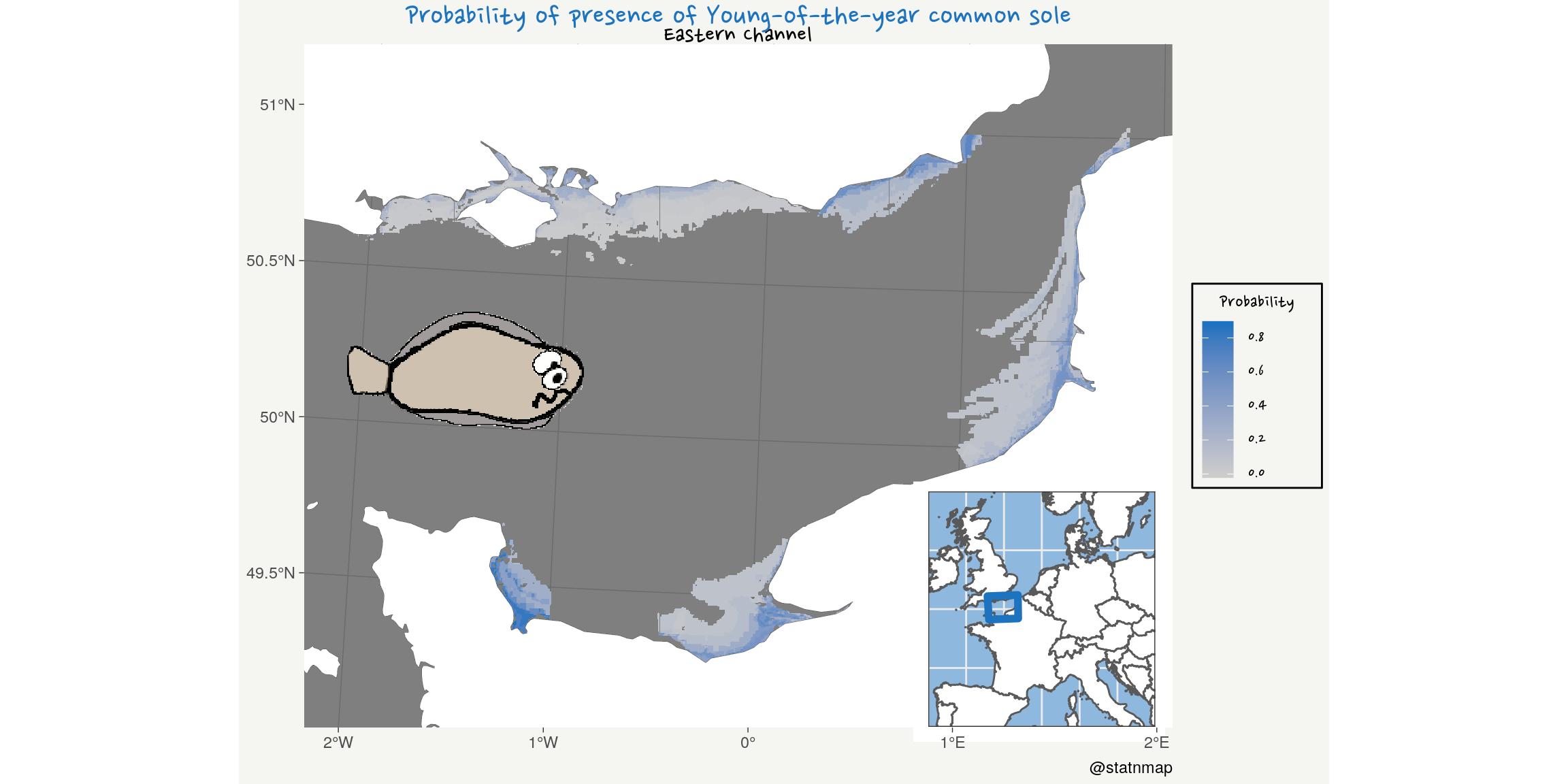
Red: Sample a polygon using a regular hexagonal grid
Where can we drink a glass of red wine in France? Let’s map the distribution of “cafes/bar” from OpenStreetMap datasets as stored by OpenDataSoft: Point of Interest in France (from OpenStreetMap).
A good opportunity to use [@Tutuchan](https://twitter.com/Tutuchan) package {fodr} to download data from French Open Data portals.
To play a little with hex, we will transform a geographical points cloud to an hexagonal grid.
We can assume a priori that distribution of bars and cafes should follow the distribution of the population. In the present case, this is exagerated by the availability of users of OpenStreetMap who complete the information. Indeed, the apparent absence of bars/cafes in some areas is more probably a consequence of the absence of OSM users, than the real absence. Because, we know that there are bars everywhere!
Here, I download data for “bar” and “cafe” separately. But there are some “cafe-bar” that should not be counted twice. I use the geographic position to merge them with {sf} and st_union.
file_bar <- file.path(extraWD, "bars.csv")
file_cafe <- file.path(extraWD, "cafes.csv")
if (!file.exists(file_bar) | !file.exists(file_cafe)) {
  # devtools::install_github("tutuchan/fodr")
  # portal <- fodr::fodr_portal("ods")
  poi <- fodr::fodr_dataset("ods", "points-dinterets-openstreetmap-en-france")

  # bars
  bars <- poi$get_records(refine = list(amenity = "bar"))

  bars_chr <- bars %>%
    dplyr::select(-geo_shape)

  write_csv(bars_chr, file_bar)

  # cafes
  cafes <- poi$get_records(refine = list(amenity = "cafe"))

  cafes_chr <- cafes %>%
    dplyr::select(-geo_shape)

  write_csv(cafes_chr, file_cafe)
} else {
  bars_chr <- read_csv(file_bar)
  cafes_chr <- read_csv(file_cafe)
}

bars_sf_l93 <- bars_chr %>%
  st_as_sf(coords = c("lng", "lat"), crs = 4326) %>%
  st_transform(crs = 2154)
cafes_sf_l93 <- cafes_chr %>%
  st_as_sf(coords = c("lng", "lat"), crs = 4326) %>%
  st_transform(crs = 2154)

cafes_bars_l93 <- rbind(bars_sf_l93, cafes_sf_l93 %>% dplyr::select(-other_tags))

# Too heavy. Rstudio breaks
# cafes_bars_union_l93 <- st_union(bars_sf_l93, cafes_sf_l93 %>% dplyr::select(-other_tags))

cafes_bars_combine_l93 <- st_union(cafes_bars_l93) %>%
  st_cast("POINT") %>%
  st_sf()

France_hex <- France_L93 %>%
  st_make_grid(what = "polygons", square = FALSE,
               n = c(40, 20)) %>%
  st_sf() %>%
  mutate(id_hex = 1:n()) %>%
  dplyr::select(id_hex, geometry)
# plot(France_hex)

# Join bars wth hex and count
bars_hex_l93 <- st_join(cafes_bars_combine_l93, France_hex)
bars_hex_count <- bars_hex_l93 %>%
  st_drop_geometry() %>%
  count(id_hex)

# Join hex with bars count
France_hex_bars <- France_hex %>%
  left_join(bars_hex_count)

ggplot(France_hex_bars) +
  geom_sf(aes(fill = n), size = 0.1) +
    scale_fill_gradient(
    high = "#AD1128", #my_blue,
    low = "grey80", na.value = NA,
    trans = "log",
    breaks = c(0, 8, 50, 400)
  ) +
  labs(
    title = "Number of cafes/bars in France",
    subtitle = "From OpenStreetMap data. Yes, this is (almost) the map of the population...",
    caption = "@statnmap - source: public.opendatasoft.com",
    x = NULL, y = NULL,
    fill = "Number"
  ) +
  coord_sf(crs = 2154) +
  my_theme()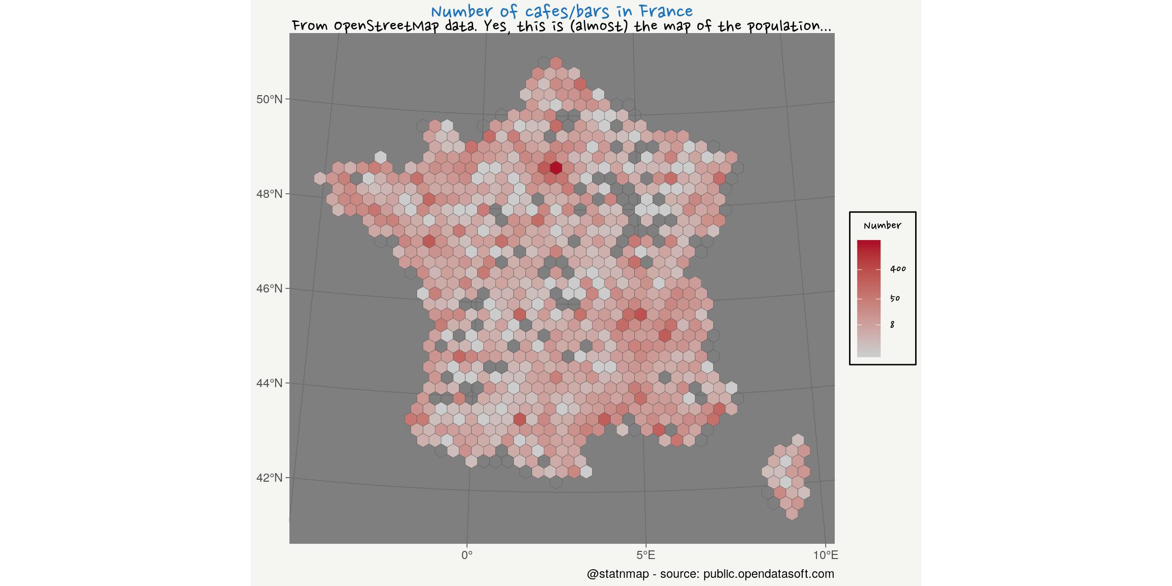
Now that you have seen possibilities of {ggplot2} to create maps with R, you can read the article of the others weeks of the challenge:
As always, code and data are available on https://github.com/statnmap/blog_tips
# Biblio with {chameleon}
tmp_biblio <- tempdir()
attachment::att_from_rmd("2019-11-08-30daymapchallenge-building-maps-1.Rmd", inside_rmd = TRUE) %>%
  chameleon::create_biblio_file(
    out.dir = tmp_biblio, to = "html", edit = FALSE)
htmltools::includeMarkdown(file.path(tmp_biblio, "bibliography.html"))
List of dependencies
- dplyr (Wickham, François, et al. (2020))
- sf (Pebesma (2020))
- raster (Hijmans (2020))
- ggplot2 (Wickham, Chang, et al. (2020))
- readr (Wickham, Hester, and Francois (2018))
- tmap (Tennekes (2020))
- extrafont (Winston Chang (2014))
- attachment (Guyader and Rochette (2020))
- chameleon (Rochette (2020))
- htmltools (RStudio and Inc. (2019))
References
Guyader, Vincent, and Sébastien Rochette. 2020. Attachment: Deal with Dependencies. https://github.com/Thinkr-open/attachment.
Hijmans, Robert J. 2020. Raster: Geographic Data Analysis and Modeling. https://CRAN.R-project.org/package=raster.
Pebesma, Edzer. 2020. Sf: Simple Features for R. https://CRAN.R-project.org/package=sf.
Rochette, Sébastien. 2020. Chameleon: Build and Highlight Package Documentation with Customized Templates. https://github.com/Thinkr-open/chameleon.
RStudio, and Inc. 2019. Htmltools: Tools for Html. https://CRAN.R-project.org/package=htmltools.
Tennekes, Martijn. 2020. Tmap: Thematic Maps. https://CRAN.R-project.org/package=tmap.
Wickham, Hadley, Winston Chang, Lionel Henry, Thomas Lin Pedersen, Kohske Takahashi, Claus Wilke, Kara Woo, Hiroaki Yutani, and Dewey Dunnington. 2020. Ggplot2: Create Elegant Data Visualisations Using the Grammar of Graphics. https://CRAN.R-project.org/package=ggplot2.
Wickham, Hadley, Romain François, Lionel Henry, and Kirill Müller. 2020. Dplyr: A Grammar of Data Manipulation. https://CRAN.R-project.org/package=dplyr.
Wickham, Hadley, Jim Hester, and Romain Francois. 2018. Readr: Read Rectangular Text Data. https://CRAN.R-project.org/package=readr.
Winston Chang. 2014. Extrafont: Tools for Using Fonts. https://CRAN.R-project.org/package=extrafont.
Citation:
For attribution, please cite this work as:
Rochette Sébastien. (2019, Nov. 08). "#30DayMapChallenge: 30 days building maps (1) - ggplot2". Retrieved from https://statnmap.com/2019-11-08-30daymapchallenge-building-maps-1/.
BibTex citation:
@misc{Roche2019#30Da,
    author = {Rochette Sébastien},
    title = {#30DayMapChallenge: 30 days building maps (1) - ggplot2},
    url = {https://statnmap.com/2019-11-08-30daymapchallenge-building-maps-1/},
    year = {2019}
  }