Play with spatial tools on 3D cells images

Use of cartography tools out of context

This won’t be the first time I use mapping tools for non-cartography purposes. In my blog post on the Shiny App for expert image comparison, I spoke about a paper written with Marion Louveaux, a bio-image data analyst working on microscopy images from plants tissues. In this paper, we used tools for mesuring spatial autocorrelation on pixel colour intensities of images from confocal microscope.
Our collaboration continues through different R-packages, in development on Marion’s github account. In this blog post, I will use outputs of 3D images issued from a cell segmentation realised by Marion with MorphoGraphX software and imported as a 3D-mesh in R thanks {mgx2r} package (here is its {pkgdown} documentation page).

I wanted to find a good reason to play with Tyler Morgan-Wall packages for 3D visualisation of raster data: {rayshader} and {rayfocus}. Using cell segmentation images in combination with {rayshader} is the challenge of the day !

library(mgx2r)
library(rgl)
library(dplyr)
library(sf)
library(ggplot2)
library(raster)
library(rayshader)
library(magick)
# extraWD <- tempdir()

Get cell segmentation dataset

We use the example data of {mgx2r} vignette. This dataset is issued from MorphoGraphX. This is a 3D surface segmentation of a 3D image. It is read and transformed as a mesh with {mgx2r} to be used with {rgl}.

By the way, I really like the new functions added to {rgl}, like this rglwidget to include {rgl} outputs in Rmarkdown HTML documents or in Shiny Apps.

This image is an interactive rgl widget

filePly <- system.file("extdata", "full/mesh/mesh_meristem_full_T0.ply", package = "mgx2r")

myMesh <- read_mgxPly(
  file = filePly, ShowSpecimen = FALSE, addNormals = TRUE,
  MatCol = 1, header_max = 30)

## [1] "Object has 7763 faces and 4158 vertices."

try(rgl.close(), silent = TRUE)
plot3d(myMesh) 
aspect3d("iso")
# Change view
view3d(theta = 30, phi = -40, zoom = 0.5)
rglwidget()

Projection and transformation as spatial object

{rayshader} requires an elevation matrix but here we have a 3D mesh. We need to project the mesh into 2 dimensions and keep the third as the elevation. By chance, the mesh is a surface mesh, which means its projection can be realised along the z-axis. For other kind of 3D mesh, I would use transform3d with a custom transformation matrix. But then, the selection of “z” for the projection will be tricky. I will not go further into this for now…

Here, as a projection, we retrieve x/y coordinates and use z as the height. This data is transformed as a spatial object with a coordinate system in meters using {sf}. If you a tutorial on {sf}, you can start with my previous blog article “Introduction to mapping with {sf} & Co.”.

mesh_sf <- t(myMesh$vb) %>% 
  as_tibble() %>% 
  st_as_sf(coords = c("x", "y"), crs = 2154)

ggplot(mesh_sf) +
  geom_sf(aes(colour = z)) +
  coord_sf(crs = 2154, datum = 2154) +
  scale_colour_gradient2(low = "#d7191c", high = "#1a9641", mid = "#ffffbf",
                         midpoint = mean(mesh_sf$z))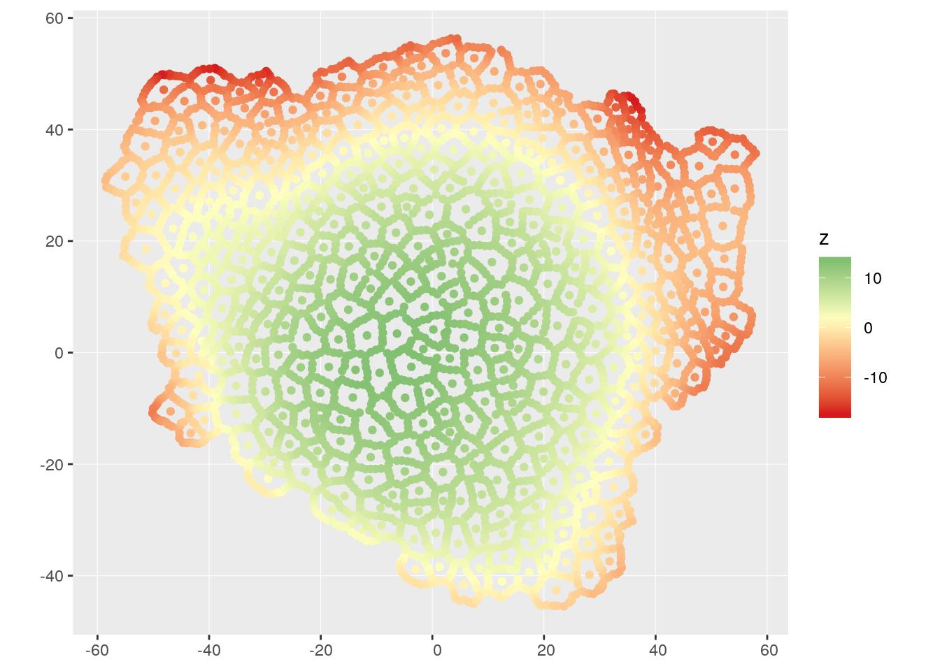

Interpolation on a raster

Our mesh transformed as spatial object is a point dataset, but {rayshader} requires a raster object. We can interpolate the mesh on a raster with inverse distance as described in my previous blog post “spatial-interpolation-on-earth-as-a-3d-sphere”.

We need a few steps:

• Create an empty raster with dimensions of the mesh
• Transform raster as spatial points with {sf}
• Calculate distance between mesh and raster points
• Proceed to inverse distance interpolation
• Set values far from data fixed to the lowest value (Avoids NA for {rayshader})
• Fill the empty raster with predictions

# Create an empty raster with dimensions of the mesh ----
r <- raster(
  as(mesh_sf, "Spatial"),
  nrows = 100, ncols = 100,
  crs = st_crs(mesh_sf)$proj4string
)

# Transform raster as spatial points with sf
r_sf <- st_as_sf(as.data.frame(coordinates(r)),
                 coords = c("x", "y"),
                   crs = 2154)

# Distance between points and raster ----
obs.r.dists <- st_distance(mesh_sf, r_sf)
obs.r.dists <- unclass(obs.r.dists)

# Inverse distance interpolation ----
## pred = 1/dist^idp
idp <- 2
inv.w <- (1/(obs.r.dists^idp))
z <- (t(inv.w) %*% matrix(mesh_sf$z)) / apply(inv.w, 2, sum)

# Remove values far from data
dist.min <- apply(obs.r.dists, 2, function(x) min(x, na.rm = TRUE))
z[dist.min > 2] <- min(z, na.rm = TRUE)

# Fill raster with predictions
r.pred <- r
values(r.pred) <- z

# Plot
rasterVis::gplot(r.pred) +
  geom_tile(aes(fill = value)) +
  scale_fill_gradient2(low = "#d7191c", high = "#1a9641", mid = "#ffffbf",
                         midpoint = mean(mesh_sf$z))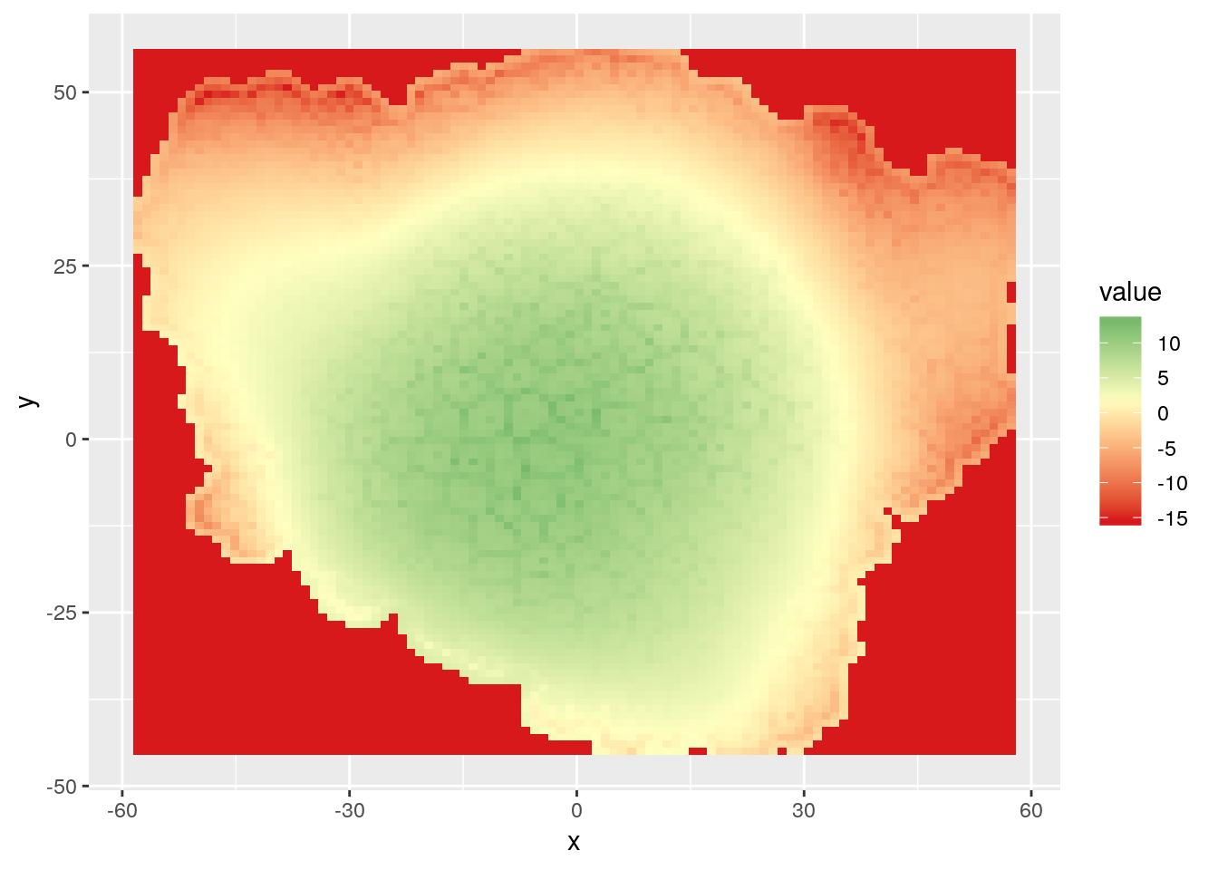

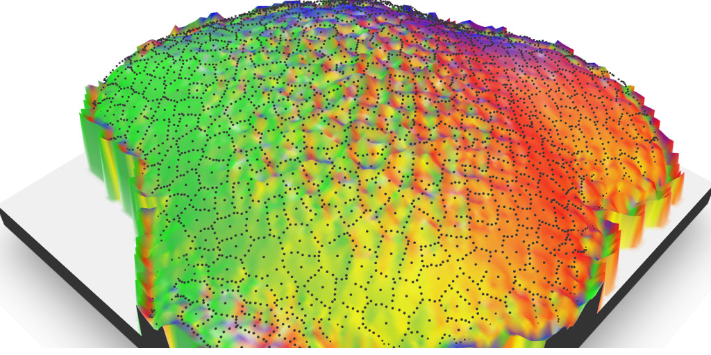
Include raster in {rayshader}

Now let’s play with {rayshader} ! To add the original points of mesh over the resulting 3D view from {rayshader}, I had to get inspiration from Neil Charles {geoviz} package that add GPS tracks to {rayshader}. This helped me determine how to use and modify x, y, z coordinated for the 3D output.

This image is an interactive rgl widget

# Transform raster as matrix for rayshader
r.matrix <- matrix(
  raster::extract(r.pred, raster::extent(r.pred)),
  nrow = ncol(r.pred),
  ncol = nrow(r.pred))

zscale <- 1

# Transform points in the scale of matrix in rayshader
mesh_sf_scale <- data.frame(st_coordinates(mesh_sf), mesh_sf$z) %>% 
  as_tibble() %>% 
  rename(z = mesh_sf.z) %>% 
  mutate(
    # X_ray = 1 * (X - xmin(r.pred)) / xres(r.pred),
    # X_ray = 1 * (X + (xmin(r.pred) + nrow(r.pred)/2)) / xres(r.pred),
    X_ray = 1 * (X + 8) / xres(r.pred),
    # Y_ray = -1 * (Y - ymin(r.pred)) / yres(r.pred),
    # Y_ray = -1 * (Y - (ymin(r.pred) + ncol(r.pred)/2)) / yres(r.pred),
    Y_ray = -1 * (Y + 4) / yres(r.pred),
    Z_ray = z*zscale + 2.5
  )

# Create shades
try(rgl.close(), silent = TRUE)
r.matrix %>%
  sphere_shade(zscale = 0.1, texture = "unicorn", progbar = FALSE) %>%
  add_shadow(ray_shade(r.matrix, zscale = 500, progbar = FALSE), 0.5) %>%
  plot_3d(r.matrix, zscale = zscale, theta = -45, zoom = 0.5, phi = 30)

# Add mesh
spheres3d(mesh_sf_scale[,c("X_ray", "Z_ray", "Y_ray")],
       col = "grey40", radius = 0.2, add = TRUE)
# Change view
view3d(theta = 30, phi = 45, zoom = 0.5)

# rgl.snapshot(filename = file.path(extraWD))
# Output html widget for Rmd
rglwidget()

Add blurr to the field of view with {rayfocus}

There is no need to transform your 3D output to add the focus view on your image. Function render_depth in {rayshader} retrieves information needed and calls {rayfocus} to create the image wanted.

render_depth(
  focus = 0.5, focallength = 10,
  bokehshape = "hex", bokehintensity = 5,
  progbar = FALSE
)

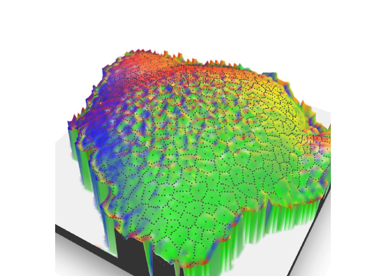
Finish with a GIF

We can not stop here after all these efforts ! Let’s have a little more fun by adding a gif to this blog post using {magick}.

seq_focus <- seq(0.4, 1, length.out = 35)
for (i in 1:length(seq_focus)) {
  view3d(theta = 30, phi = 35 + i/2, zoom = 0.5)
  
  render_depth(
    focus = seq_focus[i], focallength = 25,
    bokehshape = "hex", bokehintensity = 5,
    progbar = FALSE,
    filename = file.path(extraWD, "gif",
                         paste0(formatC(i, flag = "0", width = 3)))
  )
  
  if (i == 1) {
  all_img <- image_read(file.path(extraWD, "gif",
                         paste0(formatC(i, flag = "0", width = 3), ".png")))
  } else {
    new_img <- image_read(file.path(extraWD, "gif",
                              paste0(formatC(i, flag = "0", width = 3), ".png")))
    all_img <- c(all_img, new_img)
  }
}

# Reduce width of images
gif <- image_animate(all_img, fps = 5, loop = 0) %>% 
  image_apply(FUN = function(x) 
    image_resize(x, geometry = geometry_size_pixels(width = 500)))

# Save as gif in external directory
image_write_gif(gif, path = glue("{extraWD}/focus-1.gif"),
                delay = 0.25)

# Reduce size on disk
system(glue("convert {extraWD}/focus-1.gif -fuzz 10% -layers Optimize ../../static{StaticImgWD}/focus-low-1.gif"))

Et voilà ! I hope this blog post opens your mind on the possibilities offered by spatial tools, even if you are not doing cartography !

• {mgx2r} documentation on github.
  
• {rayshader} on github
• {rayfocus} on github

The complete R script of this article can be found on my Blog Tips Github repository.