Summary
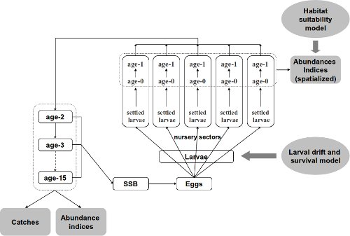
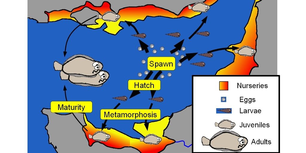
The OpenBUGS code presented below is the additional material of a publication. This is the life cycle model of a marine species (the sole in the Eastern Channel). The Bayesian hierarchical model incorporates indices of juvenile spatialized abundance, larval dispersion, adult abundance indices and catches by fishery.
Publication associated
Rochette Sebastien, Le Pape Olivier, Vigneau Joel, Rivot Etienne (2013). A hierarchical Bayesian model for embedding larval drift and habitat models in integrated life cycles for exploited fish. Ecological Applications, 23(7), 1659-1676. Publisher’s official version : http://dx.doi.org/10.1890/12-0336.1 , Open Access version : http://archimer.ifremer.fr/doc/00161/27243/

Figure 1: DAG of the Bayesian life cycle model
BUGS code to estimate parameters of a full life cycle model
- Outputs of an individual-based model for larval drift and survival that provided yearly estimates of the dispersion and mortality of eggs and larvae, from spawning grounds to settlement in several coastal nurseries;
- A habitat suitability model, based on juvenile trawl surveys coupled with a geographic information system, to estimate juvenile densities and surface areas of suitable juvenile habitat in each nursery sector;
- A statistical catch-at-age model for the estimation of the numbers-at-age and the fishing mortality on subadults and adults.
The following BUGS code refers to a specific scenario of the larvae to juvenile mortality process tested in the associated paper (see paper). This scenario (R3) assumes a density-independent mortality parameter common to all nurseries (a_BH) and a nursery-specific density-dependent mortality parameter (b_BH).
- Programmer: Sébastien Rochette, August 2012
- OpenBUGS version : 3.2.2
Inputs
- max.a: Number of age classes
- max.t: Number of years
- max.Area: Number of nurseries
- obsJuvtime : Date of observation of juvenile indices (in months)
- A_eggs, B_eggs : Fecondity parameters (at age) as Fec = exp(A_eggs + B_eggs * log(Weight-at-age))
- Pf: Female proportion (at age)
- M0: Mortality between Age 0 & Age 1 (on each area)
- M: Natural mortality (at age)
- Dij: Matrix of larval repartition among (i) Total mortality and (ii) all the areas (for each year).
- Sstar: Surface area of each area
- W_stock: Matrix of individual weights-at-age for each year
- C_obs: Matrix of observed catches-at-age for each year from age 1 to age 10
- C_obs11Plus: Vector of observed catches-at-age for each year summed for ages 11 and more
- IA_BTS_obs: Matrix of observed adult abundance indices for age 2 to max.a, for each year.
- IA_Age0: Matrix of observed age-0 abundance indices, calculated from a habitat suitability model for each year and each area.
- IA_Age1: Matrix of observed age-1 abundance indices, calculated from a habitat suitability model for each year and each area.
BUGS code:
# Bayesian Life Cycle model of a fish species
# website: http://statnmap.com

model
{

  # ----------------------------
  # Priors
  # -----------------------------

  # Catchability of BTS abundance indices (large priors)
  # Common Q for a >= 2
  Logq_0 ~ dunif(-10,10)
  Logq_1 ~ dunif(-10,10)
  Logq_AgeSup ~ dunif(-10,10)
  q_0 <- exp(Logq_0)
  q_1 <- exp(Logq_1)
  q_AgeSup <- exp(Logq_AgeSup)

  # Fishing mortality = Selectivity * Effort
  # Effort (gamma prior)
  E_Eff1 ~ dunif(0.00001, 10)
  CV_Eff ~ dunif(0.00001, 0.99999)
  a_Eff <- 1 / (CV_Eff*CV_Eff)
  b_Eff <- (1 / (CV_Eff*CV_Eff)) * (1/E_Eff1)
  for(t in 1:max.t)
  {
    Effort[t] ~ dgamma(a_Eff, b_Eff)
  }

  # Age of changing Selectivity slope (gamma prior)
  # Logistic
  CV_Selec <- 0.9
  a_Selec <- 1 / (CV_Selec * CV_Selec)
  bAge50_S <- (1 / (CV_Selec*CV_Selec)) * (1/E_Age50_S)
  bDelta_S <- (1 / (CV_Selec*CV_Selec)) * (1/E_Delta_S)
  Age50_S ~ dgamma(a_Selec,bAge50_S)
  Delta_S ~ dgamma(a_Selec,bDelta_S)
  for(a in 1:max.a)
  {
    Selec_p[a] <- (exp((2*Age50_S*log(3)/Delta_S)*(a/Age50_S-1))/(1+(exp((2*Age50_S*log(3)/Delta_S)*(a/Age50_S-1)))) )
    Selec[a] <- Selec_p[a] / Selec_p[max.a]
  }
  # Induced selectivity for abundance indices surveys
  for(a in 1:max.a) {
    SelecQ[a] <- cut(Selec[a])
    q[a] <- max(q_AgeSup * SelecQ[a] ,1.0E-7)
  }

  #Combined F=Selec*Effort (gamma prior)
  CV_F ~ dunif(0.00001, 0.99999)
  a_F <- 1 / (CV_F*CV_F)
  for(t in 1:max.t)
  {
    for(a in 1:max.a)
    {
      mean_F[a,t] <- Selec[a] * Effort[t]
      b_F[a , t] <- (1 / (CV_F*CV_F)) * (1/mean_F[a,t])
      F[a,t] ~ dgamma(a_F, b_F[a, t])
    }
    # Parameter of interest : Fishing mortality
    F3_8[t] <- mean(F[3:8,t])
  }

  # Stock-Recruitment (SR) : Beverton & Holt
  #Common a_BH & Hierarchical b_BH
  mean_aBH ~ dunif(0.00001, 4)
  CV_aBH ~ dunif(0.00001, 1)
  a_aBH <- 1/(CV_aBH*CV_aBH)
  b_aBH <- (1/(CV_aBH*CV_aBH))*(1/mean_aBH)
  a_BH ~ dgamma(a_aBH,b_aBH)

  mean_bBH ~ dunif(0.00001, 0.1)
  CV_bBH ~ dunif(0.00001, 3.5)
  a_bBH <- 1/(CV_bBH*CV_bBH)
  b_bBH <- (1/(CV_bBH*CV_bBH))*(1/mean_bBH)

  # Induced Psi & K
  Psi <- exp(-a_BH)
  for(Area in 1:max.Area){
    b_BH[Area] ~ dgamma(a_bBH,b_bBH)
    K[Area] <- a_BH/b_BH[Area] * 1/(exp(a_BH) -1)
  }

  # Process error on SR (large prior)
  log_sigma2_SR ~ dunif(-10,10)
  sigma2_SR <- exp(log_sigma2_SR)
  Tau_SR <- 1 / sigma2_SR

  # Initialisation of number of Age 1 on Areas for year 1
  # large priors according to what expected while looking at ICES data (sum(N1)<1.2E5)
  for(Area in 1:max.Area)
  {
    N1[Area,1] ~ dunif(1.0E-7, 1.0E7) # Cannot be null for cohort depletion
  }

  # Initialisation of the number at all ages for year 1 (x1000)
  # For age 1
  mean_logN1_NoSpace[1] <- log(sum(N1[,1]))
  Na1[1] ~ dlnorm(mean_logN1_NoSpace[1], Tau_P)
  N[1, 1] <- Na1[1]
  # P will be N/N[age=1,cohort] to facilitate convergence of MCMC
  P[1,1] <- 1
  # For age 2 to max.a
  for(a in 2:max.a)
  {
    Na1[a] ~ dunif(1.0E-7, 1.0E7) # Cannot be null for cohort depletion
    N[a,1] <- Na1[a]
    P[a, 1] <- 1
  }

  # Variable larval key repartition
  # Prior on the parameters of the Dirichlet distribution
  log.p.dirich[1:k] ~ dmnorm(mu.log.p[],Tau[,])
  for(i in 1:k) { p.dirich[i] <- exp(log.p.dirich[i]) } # must be positive
  # Likelihood to learn from the data Dij (14/27 years available)
  for (t in 1:max.t) { Dij[t,1:k] ~ ddirich(p.dirich[1:k]) }

  # ----------------------------
  # Population dynamics
  # ----------------------------

  # "Artificial" Process error on dynamic equations (to speed up the sampling process)
  # (correponds to a Normal variability in the natural mortality)
  Tau_P <- 1000

  for(t in 1:max.t)
  {
    # Spatialisation for Larvae, Age 0 and Age 1
    for(Area in 1:max.Area)
    {
      # Repartition of Eggs to larvae with the larval key repartition
      Larvae[Area, t] <- Eggs[t] * Dij[t,Area]

      # Berverton&Holt recruitment function --> age 0
      # R = K * S / ( So + S)
      #Sstar = Surface of nurseries
      L_star[Area,t] <- Larvae[Area,t] / Sstar[Area]
      mean_N0[Area,t] <- (Psi * K[Area] * L_star[Area,t]) / (K[Area] + Psi * L_star[Area,t]) * Sstar[Area]

      # log-normal error on Age-0 juveniles survival
      mean_logN0[Area, t] <- log(mean_N0[Area, t])
      LogN0[Area, t] ~ dnorm(mean_logN0[Area, t], Tau_SR)
      N0[Area, t] <- exp(LogN0[Area, t])

      # Survival to age 1 (quasi deterministic)
      mean_LogN1[Area, t+1] <- log(N0[Area, t] * exp(-M0[Area] * (1-(obsJuvtime/12))))
      N1[Area, t+1] ~ dlnorm(mean_LogN1[Area, t+1], Tau_P)
    } # End of Area loop

    # Sum age 1 over space (quasi deterministic)
    mean_logN1_NoSpace[t+1] <- log(sum(N1[,t+1]))
    N[1, t+1] ~ dlnorm(mean_logN1_NoSpace[t+1], Tau_P)
    # P will be N/N[age=1,cohort] to facilitate convergence of MCMC
    # such that all P[1,] = 1
    P[1, t+1] <- 1

    # Dynamic equation - Age 1 : max
    # (quasi deterministic)

    # Calculation of cohorts number
    for(a in 1:(max.a))
    {
      Row[a, t] <- step(t - a - 1) * (1) + step(a - t) * (a - t +1)
      Col[a, t] <- step(t - a - 1) * (t - a + 1) + step(a - t) * (1)
    }

    # Cohort depletion
    # P is N/N[age=1,cohort] to facilitate convergence of MCMC
    for(a in 1:(max.a-1))
    {
      log_mean_P[a + 1, t + 1] <- log(P[a,t] * exp(-M[a]-F[a,t]) )
      P[a + 1, t + 1] ~ dlnorm(log_mean_P[a + 1, t + 1], Tau_P)
      N[a +1 , t +1] <- P[a +1, t +1] * N[Row[a, t], Col[a, t]]
    }

    # Fecundity (relation weight-at-age <-> number of eggs)
    # (W_Stock = weight-at-age in data)
    for(a in 1:max.a)
    {
      Fec[a, t] <- exp(A_eggs + B_eggs * log(W_Stock[a, t] * 1000))
    }

    # SSB : Only > age 3 participate to SSB
    for(a in 1:max.a)
    {
      W_Nb[a, t] <- N[a, t] * W_Stock[a, t] * step(a - 3)
    }
    # Parameter of interest
    SSB[t] <- sum(W_Nb[,t])

    # Number of eggs (x 1000) (After a P_Period mortality ~ spawning period)
    # Only > age 3 participate to reproduction
    for(a in 1:max.a)
    {
      Nb_eggs[a, t] <- N[a, t] * exp(P_Period[t]*(-M[a]-F[a,t])) * Pf[a] * Fec[a,t] * step(a - 3)
    }

  } # end of loop on t

  # For predictions on max.t+1, we use catches and fecundity of the previous year
  for(a in 1:max.a)
  {
    Nb_eggs[a, (max.t + 1)] <- N[a, (max.t + 1)] * exp(P_Period[max.t]*(-M[a]-F[a,max.t])) * Pf[a] * Fec[a,max.t] * step(a - 3)
  }

  # ----------------------------
  # Observation equations
  # ----------------------------
  # Observation variance
  # Catches (observation variance fixed)
  # USE OF EXPERTIZE HERE
  # CV_C <- 0.2 #in data [sensitivity tested 0.1 ; 0.2 ; 0.4]
  sigma2LogC <- log(CV_C*CV_C+1)
  tauLogC <- 1/sigma2LogC
  # Under declaration [not used]
  for (a in 1:max.a) { under_declare[a] <- 1 }

  # Abundance Indices
  # Adults
  CV_IA <- sqrt(exp(sigma2LogIA)-1)
  Logsigma2LogIA ~ dunif(-10,10)
  sigma2LogIA <- exp(Logsigma2LogIA)
  tauLogIA <- 1/sigma2LogIA
  # Juveniles
  CV_IAJuv <- sqrt(exp(sigma2LogIAJuv)-1)
  Logsigma2LogIAJuv ~ dunif(-10,10)
  sigma2LogIAJuv <- exp(Logsigma2LogIAJuv)
  taulogIAJuv <- 1/sigma2LogIAJuv

  # Observations
  # Catches (X 1000)
  for(t in 1:(max.t)) {
    for(a in 1:max.a) {
      C_mean[a, t] <- under_declare[a] * (
        N[a, t] * ( F[a, t] / (F[a, t] + M[a])) * (1 - exp(-1 * (M[a] + F[a, t]))) )
      C_meancor[a, t] <- C_mean[a,t] * exp(- 0.5*sigma2LogC)
      logCmean[a,t] <- log(C_meancor[a,t])

    }
    for(a in 1:10){
      C_obs[a,t] ~ dlnorm(logCmean[a,t], tauLogC)
    }
    # Observations of catches for age>10 grouped in a 10+ group
    C_mean11Plus[t] <- sum(C_meancor[11:max.a,t])
    logC_mean11Plus[t] <- log(C_mean11Plus[t])
    C_obs11Plus[t] ~ dlnorm(logC_mean11Plus[t], tauLogC)
  }

  # Abundance indices for adults
  for(t in 1:(max.t)) {
    for(a in 2:max.a) {
      #Abundance indices including selectivity of the fishery
      #SelecQ[a] included in q[a]
      log_IA_BTS[a, t] <- log(q[a] * N[a, t])
      IA_BTS_obs[a, t] ~ dlnorm(log_IA_BTS[a, t], tauLogIA)
    }
  }

  # Abundance for juveniles
  for(Area in 1:max.Area){
    for(t in 1:max.t){
      # Estimation of N0 is at observation time with Dij
      log_N0[Area, t] <- log(q_0 * N0[Area, t])
      IA_Age0[Area, t] ~ dlnorm(log_N0[Area,t], taulogIAJuv)
      # Estimation of N1 is in January whereas observation is in September
      log_N1[Area, t] <- log(q_1 * N1[Area,t] * exp(-(M[1]+F[1,t])*(obsJuvtime/12)))
      IA_Age1[Area,t] ~ dlnorm(log_N1[Area,t], taulogIAJuv)
    }
  }

} #End of model
Citation:
For attribution, please cite this work as:
Rochette Sébastien. (2015, Jul. 23). "Bayesian life cycle model: OpenBUGS code". Retrieved from https://statnmap.com/2015-07-23-bayesian-life-cycle-model-openbugs-code/.
BibTex citation:
@misc{Roche2015Bayes,
    author = {Rochette Sébastien},
    title = {Bayesian life cycle model: OpenBUGS code},
    url = {https://statnmap.com/2015-07-23-bayesian-life-cycle-model-openbugs-code/},
    year = {2015}
  }

