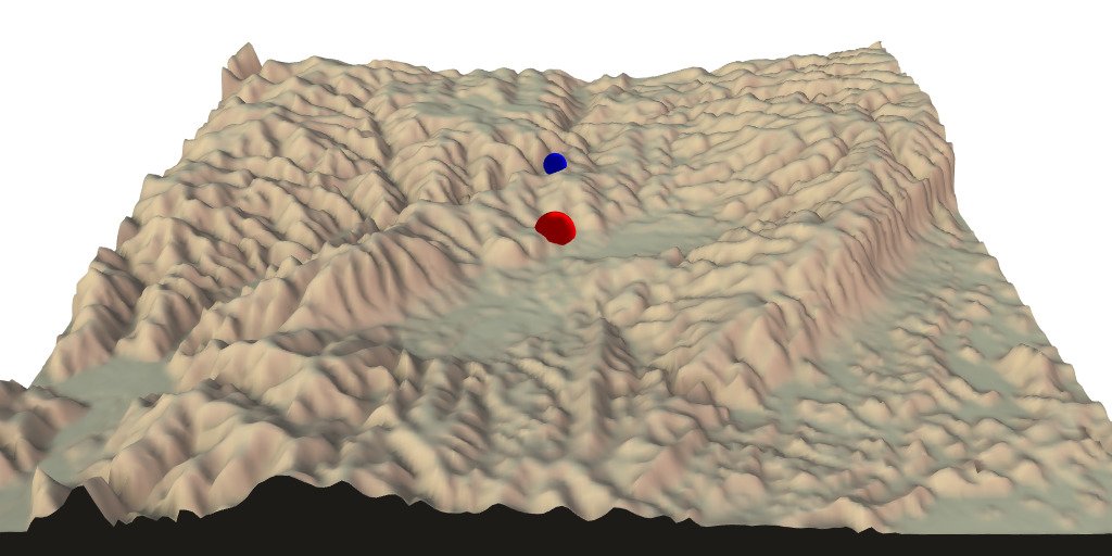
{rayshader} is a fantastic package for 3D mapping, but it comes with the limitations of {rgl}. I always found it a shame not being able to travel in all directions over my 3D objects. In this blog post, I will show a trick to simulate particle trajectory in 3 dimensions like in a “first person” video game.
Functions presented here are available in package {maps2ray} on my Github: https://github.com/statnmap/maps2ray
A few years earlier…
A few years ago, I was modelling flatfish larval dispersal in the Eastern Channel for my PhD thesis (Link to the thesis at the bottom of my CV). At that time, I dreamt I would have time to create a little video that would follow one larvae during its long journey to the coasts, then becoming a young flatfish… I never found time to do this. The only animation I could do was the following one. Symbol of the particle changes according to developmental stage of larvae. At some point, there are big enough to settle over a nursery, if reached.
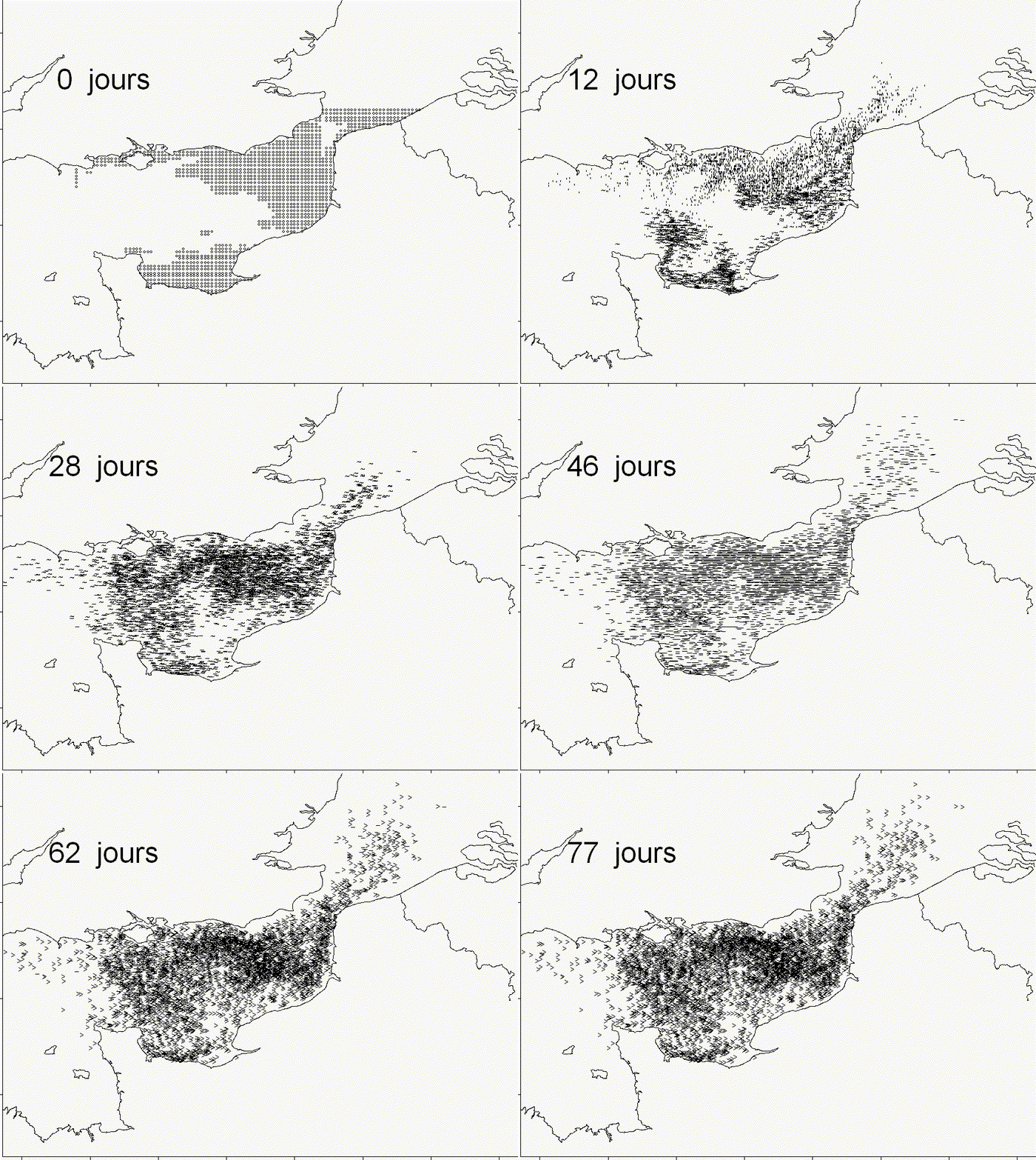
Figure 1: Solea solea larval dispersal
Now, with {rayshader}, my dreams may become true !
Packages
# devtools::install_github("tylermorganwall/rayshader")
# remotes::install_github("statnmap/mesh2ray")
library(rayshader)
library(sf)
library(raster)
library(rasterVis)
library(ggplot2)
library(dplyr)
library(rgl)
Get an altitude map
This is the map of altitude of Department ‘Loire-atlantique’ in France, downloaded from IGN website.
# extraWD <- "." # Uncomment for the script to work
if (!file.exists(file.path(extraWD, "Alti_mosaic_L93.tif"))) {
  # Download data
  githubURL <- "https://github.com/statnmap/blog_tips/raw/master/2019-10-06-follow-moving-particle-trajectory-on-raster-with-rayshader/Alti_mosaic_L93.tif"
  download.file(githubURL, destfile =  file.path(extraWD, "Alti_mosaic_L93.tif"))
}

altitude <- raster(file.path(extraWD, "Alti_mosaic_L93.tif")) # %>%
  # aggregate(fact = 2)
plot(altitude)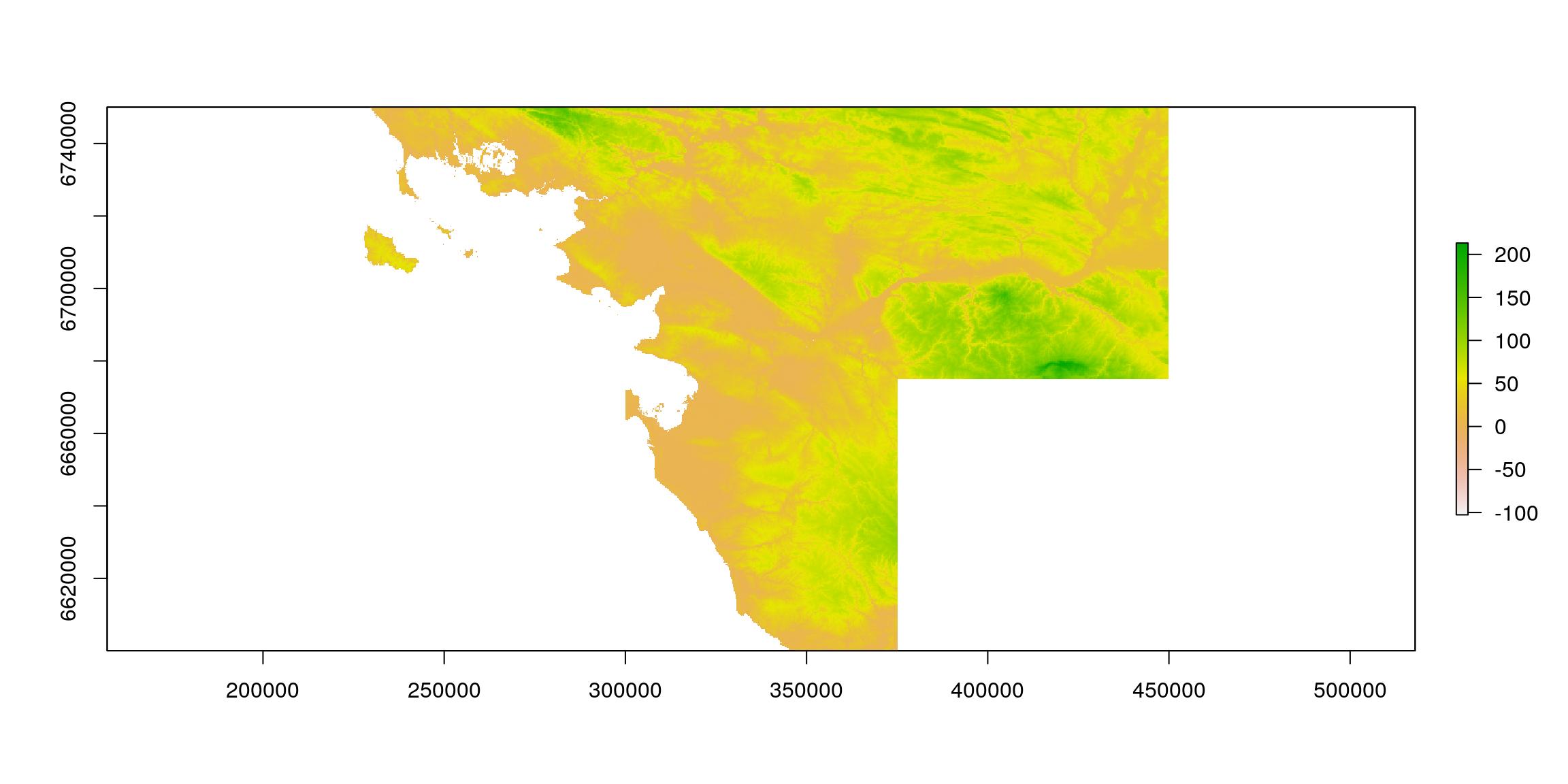
Figure 2: Loire-atlantique Altitude
Create a trajectory as {sf} spatial object
We first create a straight line that we sample regularly into points.
line_mat <- matrix(c(250000, 450000, 6720000, 6720000), ncol = 2)
line_traject <- st_linestring(x = line_mat)
point_traject <- st_sample(line_traject, size = 50, type = "regular") %>%
  st_set_crs(2154) %>%
  st_sf()

# Plot
gplot(altitude) +
  geom_tile(aes(fill = value)) +
  geom_sf(data = point_traject, colour = "white", inherit.aes = FALSE) +
  scale_fill_viridis_c()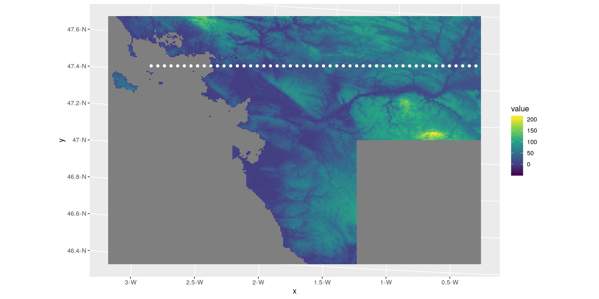
Figure 3: Simple trajectory with {sf}
Create function to transform {sf} object ready for {rayshader}
This is not a secret, I like to play with {rayshader}. Other articles of my own are here as my experiments with {rayshader}. Also, I like to play with spatial objects. For this, package {sf} is a good start.
Hence, in my talk called “Everything but maps with spatial tools” at SatRday Paris, I presented some 3D visualisations overlaid with {sf} spatial objects. I do not think I shared the script to realise this. So here it is.
You will find below a function that modifies {sf} objects to be overlaid on a {raster} object using {rayshader}: sf_proj_as_ray(). This recalculate positions in the future coordinates reference system of your raster transformed for rayshading.
This function is in package {maps2ray} on my Github: https://github.com/statnmap/maps2ray
#' Modify sf data to plot over rayshader
#'
#' @param r original raster used in rayshader
#' @param sf sf object to add on plot (with or without z column)
#' @param z_pos z-position of the sf on the 3d map if not in dataset
#' @param zscale if z-column existed in the dataset
#' @param as_sf Logical. Return sf object or not
#' @param groups Logical. Whether to group coordinates in blocks according to original structure.
#' @param crop Whether to crop sf object to extent of raster
#'
#' @export
sf_proj_as_ray <- function(r, sf, z_pos = 1, zscale = 10, as_sf = TRUE, groups = TRUE, crop = TRUE) {

  # Crop to extent of raster
  if (isTRUE(crop)) {
    sf <- st_crop(sf, st_bbox(r))
  }

  if (!is.null(sf$z)) {
    sf <- sf %>%
      mutate(
        L2 = 1:n(),
        Z_ray = z / zscale
      )
  } else {
    sf <- sf %>%
      mutate(
        L2 = 1:n(),
        Z_ray = z_pos / zscale
      )
  }

  coords <- sf %>%
    st_coordinates() %>%
    as.data.frame() %>%
    as_tibble() %>%
    mutate(
      X_ray = (X - xmin(r)) / xres(r),
      # Y_ray = -1*(Y - ymin(r)) / yres(r)
      Y_ray = 1*(Y - ymin(r)) / yres(r)
    )

  if (!"L1" %in% names(coords)) {
    coords <- coords %>%
      mutate(L1 = 1,
             L2 = 1:n()
      )
  } else if (!"L2" %in% names(coords)) {
    coords <- coords %>%
      group_by(L1) %>%
      mutate(L2 = L1,
             L1b = 1:n()) %>%
      ungroup() %>%
      mutate(L1 = L1b) %>%
      select(-L1b)
  }

  if (isTRUE(as_sf)) {
    coords_sf <- coords %>%
      select(-X, -Y) %>%
      st_as_sf(coords = c("X_ray", "Y_ray")) %>%
      group_by(L1, L2) %>%
      summarise(do_union = FALSE) %>%
      left_join(as.data.frame(sf) %>% select(-geometry))

    if (all(st_is(sf, c("POLYGON", "MULTIPOLYGON")))) {
      coords_sf <- coords_sf %>%
        st_cast("POLYGON")
    } else  if (all(st_is(sf, c("LINESTRING", "MULTILINESTRING")))) {
      coords_sf <- coords_sf %>%
        st_cast("LINESTRING")
    }else if (all(st_is(sf, c("POINT", "MULTIPOINT")))) {
      coords_sf <- coords_sf %>%
        st_cast("POINT")
    }
  }
  if (isTRUE(groups)) {
    coords_grp <- coords %>%
      mutate(Y_ray = -1 * Y_ray) %>%
      left_join(st_drop_geometry(sf)) %>%
      group_by(L1, L2) %>%
      tidyr::nest(coords = c(X_ray, Z_ray, Y_ray))
  }

  if (isTRUE(as_sf) & isTRUE(groups)) {
    res <- list(sf = coords_sf, coords = coords_grp)
  } else if (isTRUE(as_sf) & !isTRUE(groups)) {
    res <- list(sf = coords_sf, coords = coords)
  } else if (isTRUE(as_sf) & !isTRUE(groups)) {
    res <- list(coords = coords_grp)
  } else {
    res <- list(coords = coords)
  }
  return(res)
}
Show points over raster in rayshader
Now, you can plot outputs of the function.
- Calculate {sf} object coordinates in future rayshader coordinates system using
sf_proj_as_ray()- Define
zscale <- 10for all {rayshader} objects
- Define
zscale <- 5
points_ray <- sf_proj_as_ray(r = altitude, sf = point_traject,
                             z_pos = maxValue(altitude) + 10,
zscale = zscale)- Create the {rayshader} terrain object to be used in both 2D and 3D outputs
# Transform raster as matrix
datamat <- t(as.matrix(altitude))
# Rayshade raster
ambmat <- ambient_shade(datamat, zscale = zscale)
raymat <- ray_shade(datamat, zscale = zscale, lambert = TRUE)

# Create ray_image
ray_image <- datamat %>%
  sphere_shade(texture = "imhof4") %>%
  add_shadow(raymat, max_darken = 0.5) %>%
add_shadow(ambmat, max_darken = 0.5) - Plot rayshader image in 2D and add points with new coordinates reference system of {rayshader}:
sflist in the output ofsf_proj_as_ray().- The red point is a target for the following paragraphs
# plot rayshader in 2D
plot_map(ray_image)
plot(points_ray$sf, col = "blue", pch = 20, add = TRUE, reset = FALSE)
plot(points_ray$sf[10,], col = "red", pch = 20, cex = 2, add = TRUE, reset = FALSE)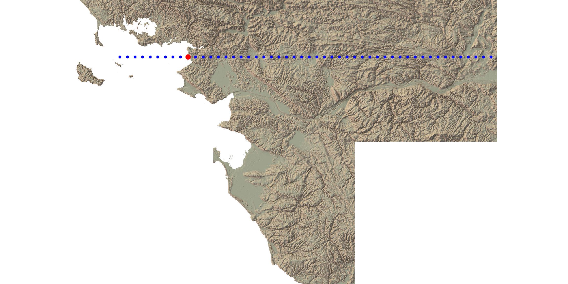
Figure 4: Trajectory over {rayshader} in 2D
- Plot {rayshader} image in 3D and overlay points with the new coordinates reference system of {rayshader}:
coordslist in the output ofsf_proj_as_ray().
ray_image %>%
  plot_3d(
    datamat,
    zscale = zscale, windowsize = c(500, 500),
    soliddepth = -max(datamat, na.rm = TRUE)/zscale,
    water = TRUE, wateralpha = 0,
    theta = 15, phi = 40,
    zoom = 0.6,
    fov = 60)

spheres3d(
  bind_rows(points_ray$coords$coords),
  col = "blue", add = TRUE, radius = 10,
  alpha = 1)

i <- 10
spheres3d(
  points_ray$coords$coords[[i]],
  col = "red", add = TRUE, radius = 20,
  alpha = 1)

rgl::snapshot3d(file.path(extraWD, "ray3dtotal.png"))
rgl::rgl.close()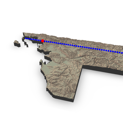
Figure 5: Trajectory over {rayshader} in 3D
Show a cropped areas
The raster is already rayshaded. If I want to zoom on a specific area, I do not want to calculate again the shading. I thus explored the reference system to crop matrices and recalculate point position on a smaller part of the raster.
To do so, I focus on one point of the trajectory (the red one above) and create a smaller window around this point.
- We can verify the correct cropping in 2D
# plot rayshader in 2D
dim(ray_image)
dim(datamat)
# Need a matrix without zero for render_label
data1 <- datamat
data1[is.na(data1)] <- 0

# Point as reference
i <- 10
position <- points_ray$coords$coords[[i]]
window <- 100
# Create a window around point
bounds <- tibble(
    Xmin = max(round(position)[1] - window, 0), # X
    Xmax = min(round(position)[1] + window, dim(datamat)[1]),
    Ymin_pos = max(round(position)[3] - window, -dim(datamat)[2]), # Y
    Ymax_pos = min(round(position)[3] + window, 0),
    Ymin_row = dim(datamat)[2] + Ymin_pos + 1,
    Ymax_row = dim(datamat)[2] + Ymax_pos + 1
)

# Height of the block (min - 1/5 of total height) to correct z
# soliddepth <- min(datamat, na.rm = TRUE))/zscale)
one_5 <- (max(datamat, na.rm = TRUE) - min(datamat, na.rm = TRUE))/5
soliddepth <- (min(datamat, na.rm = TRUE) - one_5)/zscale

# Calculate new position of the point on the cropped raster
position_bounds <- position %>%
  mutate(
    X_ray = X_ray - bounds$Xmin + 1,
    Y_2d = Y_ray - bounds$Ymin_pos + 1,
    Y_ray = -1 * (Y_ray - bounds$Ymin_pos + 1),
    Z_ray = Z_ray
  )

# Verify cropped area and point position
plot_map(ray_image[bounds$Ymin_row:bounds$Ymax_row,bounds$Xmin:bounds$Xmax,])
points(position_bounds[,c("X_ray", "Y_2d")], col = "red", pch = 20, cex = 2)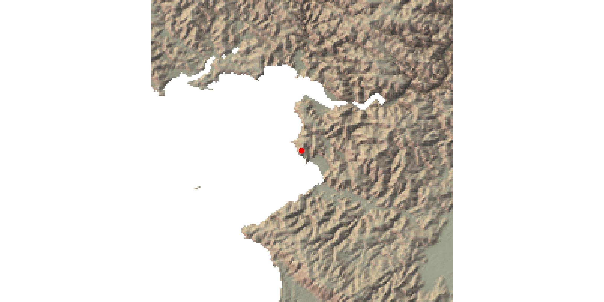
Figure 6: Verify cropping area in {rayshader} 2D
- Then in 3D
ray_image[bounds$Ymin_row:bounds$Ymax_row,bounds$Xmin:bounds$Xmax,] %>%
  plot_3d(
    datamat[bounds$Xmin:bounds$Xmax, bounds$Ymin_row:bounds$Ymax_row],
    zscale = zscale, windowsize = c(500, 500),
    soliddepth = soliddepth,
    water = TRUE, wateralpha = 0,
    theta = -90, phi = 30,
    zoom = 0.4,
    fov = 80)

render_label(
  data1[bounds$Xmin:bounds$Xmax, bounds$Ymin_pos:bounds$Ymax_pos],
  x = pull(position_bounds[1, "X_ray"]),
  y = -pull(position_bounds[1, "Y_ray"]),
  z = 200,
  zscale = zscale,
  text = "Here",
  color = "red"
)

spheres3d(position_bounds[,c("X_ray", "Z_ray", "Y_ray")],
          color = "red", add = TRUE, lwd = 5, radius = 5,
          alpha = 1)

rgl::snapshot3d(file.path(extraWD, "ray3dcrop.png"))
rgl::rgl.close()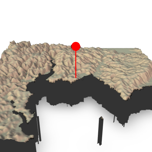
Figure 7: Trajectory over {rayshader} in 3D
What about playing a film now ?
I can create the scenes around each point of the trajectory and follow this sphere over the scene in a gif.
- Let’s put everything together in a function
This function is in package {maps2ray} on my Github: https://github.com/statnmap/maps2ray
#' Create a cropped scene
#'
#' @param datamat Original raster transformed as matrix with t(as.matrix(raster))
#' @param ray_image Rayshaded image created with sphere_shade, add_shadow, ...
#' @param position dataframe of point coordinates in the {rayshader} system
#' as created using sf_proj_as_ray()
#' @param position_next dataframe of another point coordinates in the {rayshader}
#'system as created using sf_proj_as_ray()
#' @param window size of the square window in pixels around the position
#' @param zscale Ratio between Z and x/y. Adjust the zscale down to exaggerate
#' elevation features. Better to use the same for the entire workflow.
#' @param zoom Zoom factor. Reduce to zoom in.
#' @param windowsize Size of the rgl window
render_cropped_scene <- function(ray_image, datamat, position,
                                 position_next,
                                 window = 100,
                                 zscale = 5, zoom = 0.4,
                                 windowsize = c(500, 500)) {
  # Create a window around point
  bounds <- tibble(
    Xmin = max(round(position)[1] - window, 0), # X
    Xmax = min(round(position)[1] + window, dim(datamat)[1]),
    Ymin_pos = max(round(position)[3] - window, -dim(datamat)[2]), # Y
    Ymax_pos = min(round(position)[3] + window, 0),
    Ymin_row = dim(datamat)[2] + Ymin_pos + 1,
    Ymax_row = dim(datamat)[2] + Ymax_pos + 1
  )

  # Height of the block (min - 1/5 of total height) to correct z
  # soliddepth <- min(datamat, na.rm = TRUE))/zscale)
  one_5 <- (max(datamat, na.rm = TRUE) - min(datamat, na.rm = TRUE))/5
  soliddepth <- (min(datamat, na.rm = TRUE) - one_5)/zscale

  # Calculate new position of the point on the cropped raster
  position_bounds <- position %>%
    mutate(
      X_ray = X_ray - bounds$Xmin + 1,
      Y_2d = Y_ray - bounds$Ymin_pos + 1,
      Y_ray = -1 * (Y_ray - bounds$Ymin_pos + 1),
      Z_ray = Z_ray #/zscale
    )

  # Plot cropped 3D output
  ray_image[bounds$Ymin_row:bounds$Ymax_row,bounds$Xmin:bounds$Xmax,] %>%
    plot_3d(
      datamat[bounds$Xmin:bounds$Xmax, bounds$Ymin_row:bounds$Ymax_row],
      zscale = zscale, windowsize = windowsize,
      # soliddepth = -min(datamat, na.rm = TRUE)/zscale,
      soliddepth = soliddepth,
      water = TRUE, wateralpha = 0,
      theta = -90, phi = 30,
      zoom = zoom,
      fov = 80)

  # Add point at position
  spheres3d(position_bounds[,c("X_ray", "Z_ray", "Y_ray")],
            color = "red", add = TRUE, lwd = 5, radius = 5,
            alpha = 1)

  if (!missing(position_next)) {
    position_next_bounds <- position_next %>%
      mutate(
        X_ray = X_ray - bounds$Xmin + 1,
        Y_2d = Y_ray - bounds$Ymin_pos + 1,
        Y_ray = -1 * (Y_ray - bounds$Ymin_pos + 1),
        Z_ray = Z_ray
      )

    # Add point at position
    spheres3d(position_next_bounds[,c("X_ray", "Z_ray", "Y_ray")],
              color = "blue", add = TRUE, lwd = 5, radius = 3,
              alpha = 1)
  }
}- Create a film using all positions of the trajectory
path_gif <- file.path(extraWD, "film_follow_trajectory.gif")
if (!file.exists(path_gif)) {

  # Number of frame = Number of points
  n_frames <- length(points_ray$coords$coords)
  savedir <- file.path(extraWD, "film_follow_trajectory")
  if (!dir.exists(savedir)) {
    dir.create(savedir, showWarnings = FALSE)
  }
  img_frames <- file.path(
    savedir,
    paste0("film_", formatC(seq_len(n_frames), width = 3, flag = "0"), ".png")
  )

  # create all frames
  for (i in seq_len(n_frames)) {
    # i <- 20
    position <- points_ray$coords$coords[[i]]
    if (i < n_frames) {
      position_next <- points_ray$coords$coords[[i + 1]]
      render_cropped_scene(ray_image, datamat, position,
                           position_next)
    } else {
      # Last one
      render_cropped_scene(ray_image, datamat, position)
    }
    # Save img
    rgl::snapshot3d(img_frames[i])
    rgl::clear3d()
  }
  rgl::rgl.close()

  # Create gif
  magick::image_write_gif(magick::image_read(img_frames),
                          path = path_gif,
                          delay = 6/n_frames)
}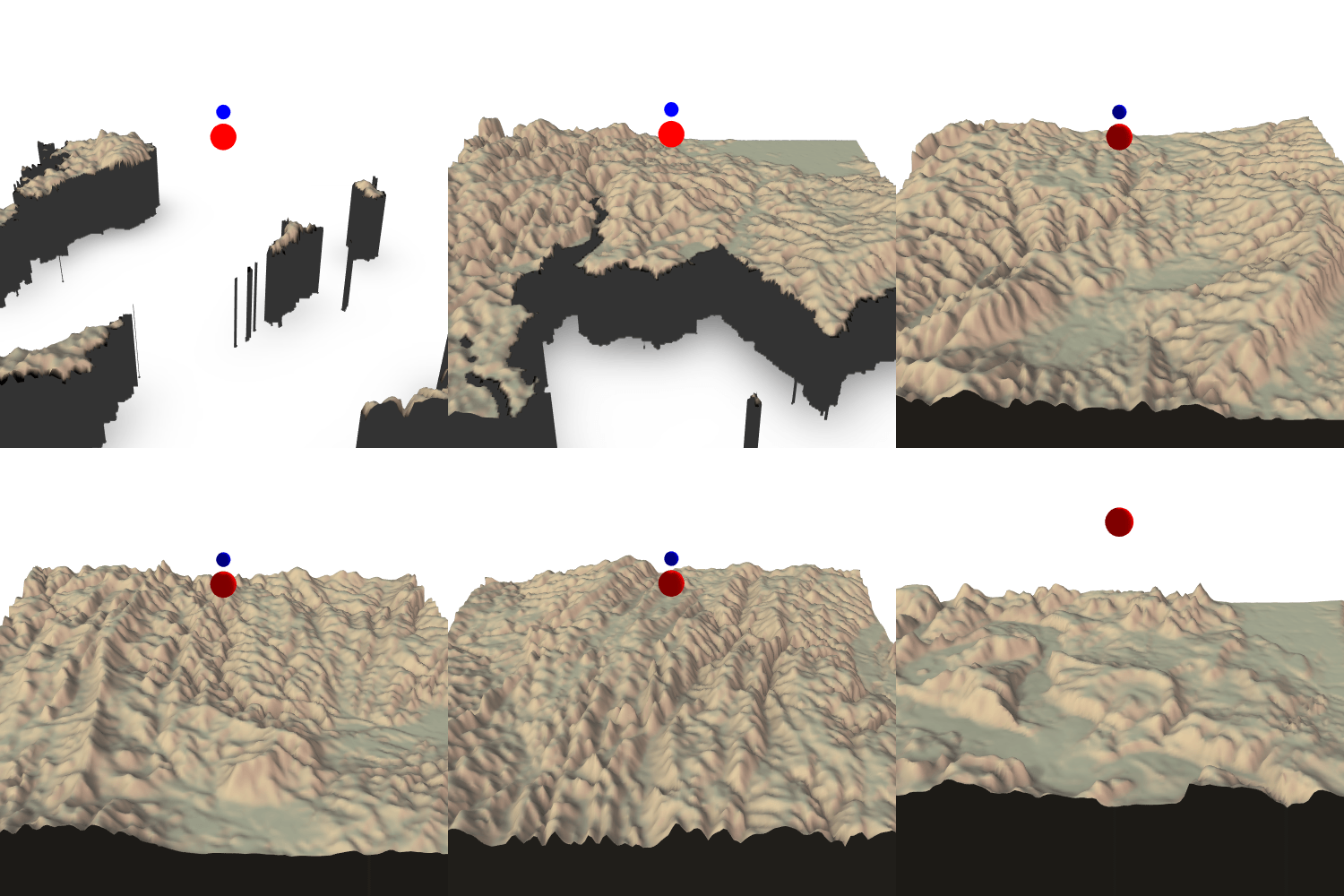
Figure 8: Film of trajectory over {rayshader} in 3D
Add points with real altitudes
- Extract altitudes at points position to be used in the film
- Recalculate positions with the {rayshader} coordinates reference system
- Build the film !
# Extract z
point_traject_z <- point_traject %>%
  st_cast("POINT") %>%
  mutate(z = raster::extract(altitude, point_traject %>% st_cast("POINT")),
         z = ifelse(is.na(z), 4, z + 1))

points_ray_z <- sf_proj_as_ray(r = altitude, sf = point_traject_z,
                             zscale = zscale)

# Create film
path_gif_alt <- file.path(extraWD, "film_follow_trajectory_altitude.gif")
if (!file.exists(path_gif_alt)) {

  # Number of frame = Number of points
  n_frames <- length(points_ray_z$coords$coords)
  savedir <- file.path(extraWD, "film_follow_trajectory_altitude")
  if (!dir.exists(savedir)) {
    dir.create(savedir, showWarnings = FALSE)
  }
  img_frames <- file.path(
    savedir,
    paste0("film_", formatC(seq_len(n_frames), width = 3, flag = "0"), ".png")
  )

  # create all frames
  for (i in seq_len(n_frames)) {
    # i <- 20
    position <- points_ray_z$coords$coords[[i]]
    if (i < n_frames) {
      position_next <- points_ray_z$coords$coords[[i + 1]]
      render_cropped_scene(ray_image, datamat, position,
                           position_next)
    } else {
      # Last one
      render_cropped_scene(ray_image, datamat, position)
    }
    # Save img
    rgl::snapshot3d(img_frames[i])
    rgl::clear3d()
  }
  rgl::rgl.close()

  # Create gif
  magick::image_write_gif(magick::image_read(img_frames),
                          path = path_gif_alt,
                          delay = 6/n_frames)
}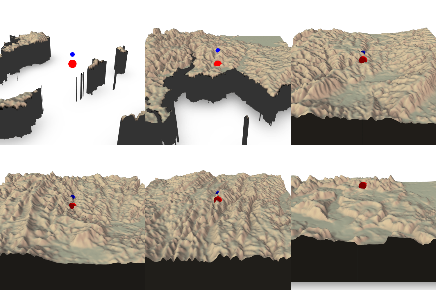
Figure 9: Film of trajectory over {rayshader} in 3D
Go further
Find the script of this blog post on my github: https://github.com/statnmap/blog_tips
Functions presented here are available in package {maps2ray} on my Github: https://github.com/statnmap/maps2ray
Now, I am waiting for other people to transform this as a video game in a Shiny Application !
- Play with {rayshader}: follow the guide.
- Follow my introduction to mapping using package {sf}
- Discover my other explorations of {rayshader}
- Learn cartography in R directly with me
# For header
i <- 20
position <- points_ray_z$coords$coords[[i]]
position_next <- points_ray_z$coords$coords[[i + 1]]
render_cropped_scene(ray_image, datamat, position,
                     position_next, windowsize = c(1024, 512),
                     zoom = 0.3)

rgl::snapshot3d(file.path(extraWD, paste0(slug, "_header.png")))
Citation:
For attribution, please cite this work as:
Rochette Sébastien. (2019, Oct. 06). "Follow moving particle trajectory over raster with {rayshader}". Retrieved from https://statnmap.com/2019-10-06-follow-moving-particle-trajectory-on-raster-with-rayshader/.
BibTex citation:
@misc{Roche2019Follo,
    author = {Rochette Sébastien},
    title = {Follow moving particle trajectory over raster with {rayshader}},
    url = {https://statnmap.com/2019-10-06-follow-moving-particle-trajectory-on-raster-with-rayshader/},
    year = {2019}
  }

