Mapping, spatial analyses and GIS with R

Some slides to present GIS with R

If you download the following presentation, you will find a presentation of different functions in the R-software useful for spatial data manipulations. Choosing the right libraries allows to create, import, modify, manipulate and map vector (shapefiles) or matrix (raster) spatial data. Your spatial files can then be used for modeling and spatial interpolation like kriging.

If you want to know more about gis and mapping with R, I can propose a tutorial

The presentation can be downloaded here, however, this presentation is in French, although images and r-code provided is normally clear enough for anybody to understand. The R-code used to create images for this presentation is on my github

This presentation has been realized in 2012. There may be some modifications in functions presented. For instance, in library “sp”, fonction overlay() in now called over().

# R-code for spatial joint between points and polygons
# website: http://statnmap.com

library(sp)
library(rgdal)
library(raster)
library(dismo) # For googlemap as raster object

# Raster Map with the extent of the study area: "RastStudy"
# Get Google Map
g <- gmap('Treffiagat, Bretagne, France', type = 'roadmap', exp = 5)

# Draw manually polygons on the map
mpol <- drawPoly(sp = FALSE, col = "black", lwd = 2)
mpol2 <- drawPoly(sp = FALSE, col = "red", lwd = 2)
mpol3 <- drawPoly(sp = FALSE, col = "pink", lwd = 2)
# Create a SpatialPolygon from multiple polygons
P1 <- SpatialPolygons(
  list(Polygons(list(Polygon(mpol), Polygon(mpol3)), "type1"),
       Polygons(list(Polygon(mpol2)), "type2")))

# Define manually points on the map and transform as SpatialPoints
pt <- locator(n = 10, type = "p", col = "black", pch = 20)
pt <- data.frame(x = pt$x, y = pt$y)
pt <- SpatialPoints(pt, proj4string = 
                      CRS("+proj=merc +a=6378137 +b=6378137 +lat_ts=0.0 +lon_0=0.0 +x_0=0.0 +y_0=0 +k=1.0 +units=m +nadgrids=@null +no_defs"))

# Spatial join of points and polygons
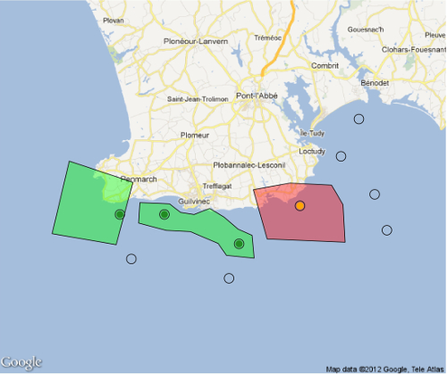
pt_label <- over(pt,P1)

# Figure
jpeg(filename = "overlay_polygon.jpeg",
     width = 20, height = 20, units = "cm", pointsize = 5,
     quality = 100,
     bg = "white", res = 300)  
  plot(g)
  plot(P1, add = TRUE,
       col = c(rgb(0, 255, 0, 100, maxColorValue = 255),
               rgb(255, 0, 0, 100, maxColorValue = 255)))
  plot(pt, cex = 5, add = TRUE, pch = 1)
  # Color points according to polygon label
  plot(pt[which(pt_label == 1),], col = "forestgreen", cex = 5, add = TRUE, pch = 20)
  plot(pt[which(pt_label == 2),], col = "orange", cex = 5, add = TRUE, pch = 20)
dev.off()

Figure 1: Spatial joint between points and polygons using R-software

# Produce a raster of prediction from stack and model
predfun <- function(model, data, sefit=FALSE) {
  v <- predict(model, data, se.fit = TRUE, type = "response")
  if (!sefit) {
    p <- as.vector(v$fit)
  } else {
    p <- as.vector(v$se.fit)
  }
  p
}
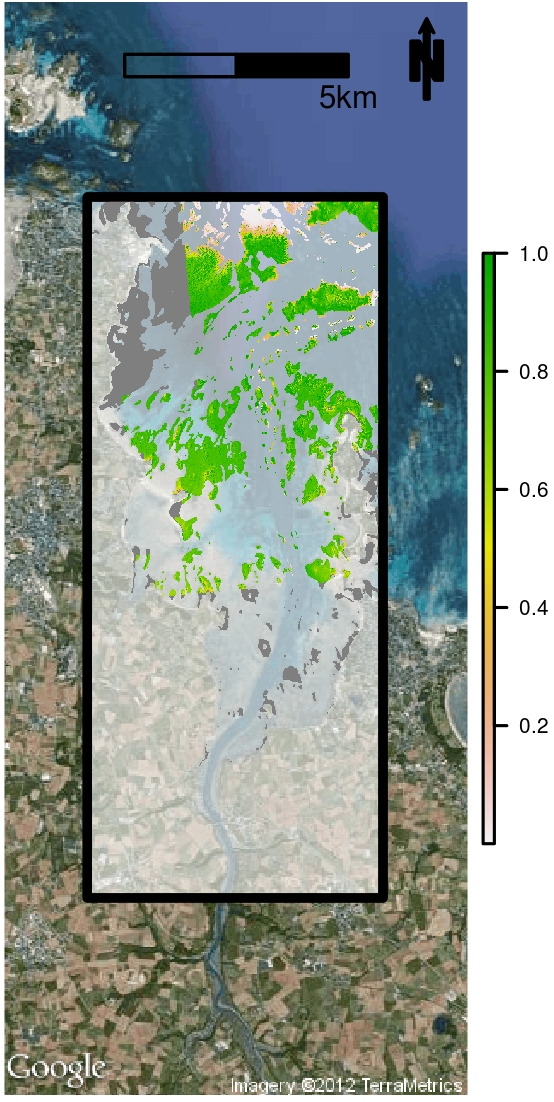
predmap <- raster::predict(RasterForPred, model=model, fun=predfun, sefit=FALSE, index=1)
predmap.se <- ratser::predict(RasterForPred, model=model, fun=predfun, sefit=TRUE, index=1)

Figure 2: Output of spatial distribution modelling using R-software