Cartographie, analyses spatiales et SIG avec R

Une présentation des SIG avec R

En cliquant sur le lien ci-dessous, vous trouverez une présentation balayant différentes fonctions du logiciel R utiles lorsque l’on souhaite travailler avec des jeux de données spatialisées et faire des opérations de SIG. Les bonnes libraries du logiciel R vous permettent de créer, importer, modifier, manipuler et cartographier des fichiers spatialisés vectoriels (shapefiles) ou matriciels (rasters). Vos fichiers spatialisés peuvent ensuite être utilisés pour faire de la modélisation ou de l’interpolation spatiale (krigeage).

Si vous souhaitez en savoir plus, je peux vous proposer une formation aux sig avec R. La présentation est à télécharger ici. Le script R utilisé pour créer les figures de cette présentation est disponible sur mon github.

La présentation date de 2012. Il y a pu y avoir quelques modifications dans les fonctions. Par exemple, dans la librairie “sp”, la fonction overlay() s’appelle désormais over().

# R-code for spatial joint between points and polygons
# website: http://statnmap.com

library(sp)
library(rgdal)
library(raster)
library(dismo) # For googlemap as raster object

# Raster Map with the extent of the study area: "RastStudy"
# Get Google Map
g <- gmap('Treffiagat, Bretagne, France', type = 'roadmap', exp = 5)

# Draw manually polygons on the map
mpol <- drawPoly(sp = FALSE, col = "black", lwd = 2)
mpol2 <- drawPoly(sp = FALSE, col = "red", lwd = 2)
mpol3 <- drawPoly(sp = FALSE, col = "pink", lwd = 2)
# Create a SpatialPolygon from multiple polygons
P1 <- SpatialPolygons(
  list(Polygons(list(Polygon(mpol), Polygon(mpol3)), "type1"),
       Polygons(list(Polygon(mpol2)), "type2")))

# Define manually points on the map and transform as SpatialPoints
pt <- locator(n = 10, type = "p", col = "black", pch = 20)
pt <- data.frame(x = pt$x, y = pt$y)
pt <- SpatialPoints(pt, proj4string = 
                      CRS("+proj=merc +a=6378137 +b=6378137 +lat_ts=0.0 +lon_0=0.0 +x_0=0.0 +y_0=0 +k=1.0 +units=m +nadgrids=@null +no_defs"))

# Spatial join of points and polygons
pt_label <- over(pt,P1)

# Figure
jpeg(filename = "overlay_polygon.jpeg",
     width = 20, height = 20, units = "cm", pointsize = 5,
     quality = 100,
     bg = "white", res = 300)  
  plot(g)
  plot(P1, add = TRUE,
       col = c(rgb(0, 255, 0, 100, maxColorValue = 255),
               rgb(255, 0, 0, 100, maxColorValue = 255)))
  plot(pt, cex = 5, add = TRUE, pch = 1)
  # Color points according to polygon label
  plot(pt[which(pt_label == 1),], col = "forestgreen", cex = 5, add = TRUE, pch = 20)
  plot(pt[which(pt_label == 2),], col = "orange", cex = 5, add = TRUE, pch = 20)
dev.off()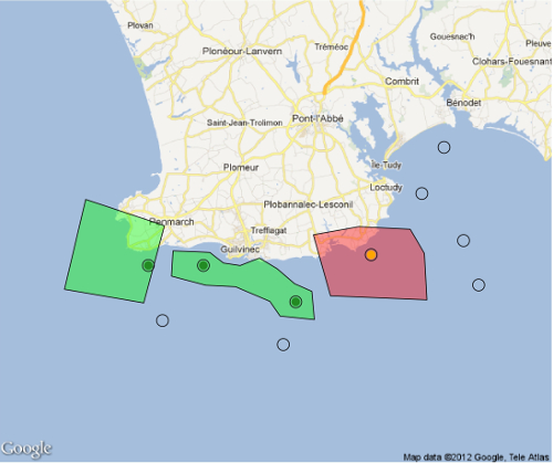

Figure 1: Jointure spatiale entre points et polygones avec le logiciel R

# Produce a raster of prediction from stack and model
predfun <- function(model, data, sefit=FALSE) {
  v <- predict(model, data, se.fit = TRUE, type = "response")
  if (!sefit) {
    p <- as.vector(v$fit)
  } else {
    p <- as.vector(v$se.fit)
  }
  p
}
predmap <- raster::predict(RasterForPred, model=model, fun=predfun, sefit=FALSE, index=1)
predmap.se <- ratser::predict(RasterForPred, model=model, fun=predfun, sefit=TRUE, index=1)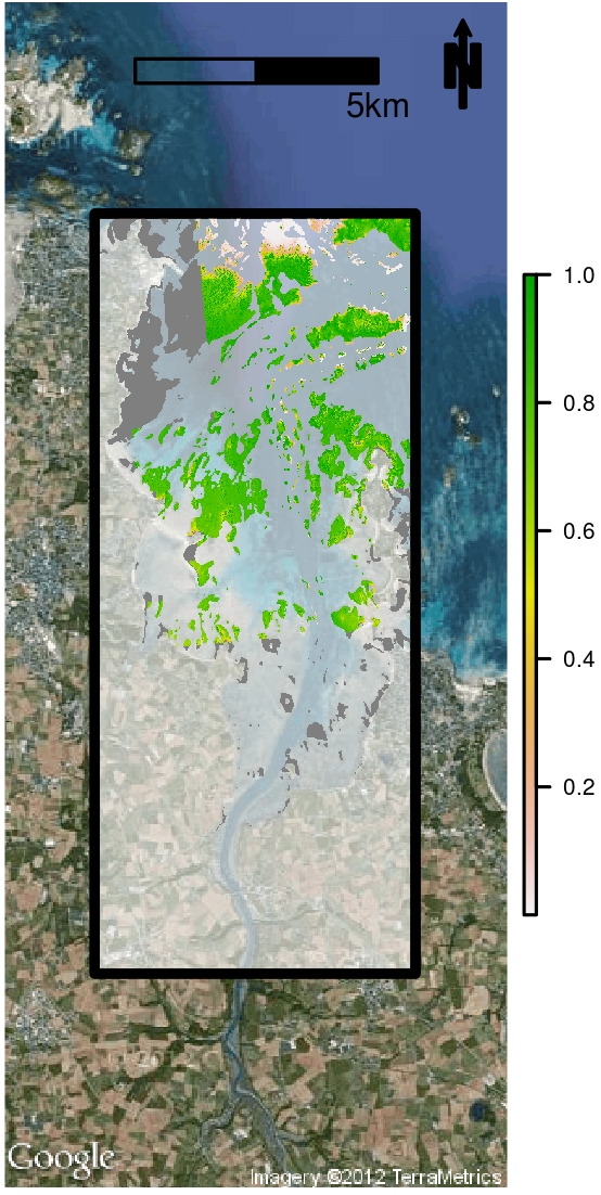

Figure 2: Prédictions d’un modèle de distribution d’espèce à l’aide du logiciel R