Plot a specific image in a delimited polygon as repeated pattern on a map

Symbology for mapping with R

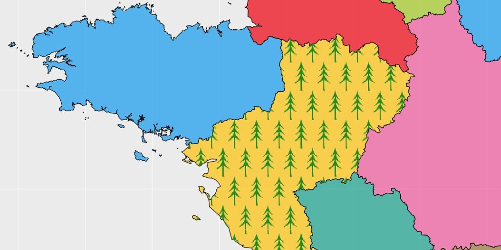
A question on stackoverflow asked how to draw trees in a polygon to represent a forest area on a map. I first thought about plotting “emoji” on a regular point pattern sampled in the polygon. Library sp allows for sampling points in a delimited SpatialPolygons which was exactly what I was looking for. I also thought about the possibility to plot y own image, which is possible using function rasterImage. Here, we will go further with GIS symbology for polygons with Rstats. We also create a function a little more advanced than rasterImage. The complete script is here.

Some data

Let us define a SpatialPolygonsDataFrame to work on. Let’s also define the specific polygon in which to draw the forest.

# Load global map
fra.sp.orig <- getData('GADM', country = 'FRA', level = 1, path = extraWD)
fra.sp <- gSimplify(fra.sp.orig, tol = 0.005) %>%
  SpatialPolygonsDataFrame(data = data.frame(NAME = fra.sp.orig$NAME_1))

# Select polygon in which adding symbols
pol <- fra.sp[which(fra.sp$NAME == "Pays de la Loire"),]

# Define extent for figures
e <- extend(extent(pol), c(2.75, 1.6, 1.3, 1.5))
ext.pol <- SpatialPolygons(list(Polygons(list(Polygon(
  rbind(c(e@xmin, e@ymin), c(e@xmin, e@ymax), 
        c(e@xmax, e@ymax), c(e@xmax, e@ymin),
        c(e@xmin, e@ymin)))), ID = 1)))
proj4string(ext.pol) <- proj4string(fra.sp)

# Define colors fixed for some regions
col.n <- c(9,1,4,2,3,6,4,5,5,6,7,6,7,10,7,3,9,8,7,9,7,1)
col.region <- yarrr::piratepal("basel")[col.n]

###Draw a point grid with emoji in a specific polygon

We can sample points in the polygon area using sp::spsample function. We can then plot at the coordinates locations, any emoji using library emojifont for instance.

# Create a point grid in a specific polygon -----------------------------------
grid.pt <- sp::spsample(pol, n = 25, type = "regular")

par(mai = c(0, 0, 0, 0))
# plot the entire map with restricted limits
plot(ext.pol, xaxs = "i", yaxs = "i", border = NA)
plot(fra.sp, col = scales::alpha(col.region, alpha = 0.7), add = TRUE)
# Highlight the selected polygon
plot(pol, border = "red", lwd = 3, add = TRUE)
# Normal points
points(grid.pt, pch = 20, col = "blue", cex = 0.1)
# Add emojifont instead of points
text(coordinates(grid.pt)[, 1], coordinates(grid.pt)[, 2],
     labels = emoji('evergreen_tree'), cex = 2, lwd = 3,
     col = 'forestgreen', family = 'OpenSansEmoji')
box()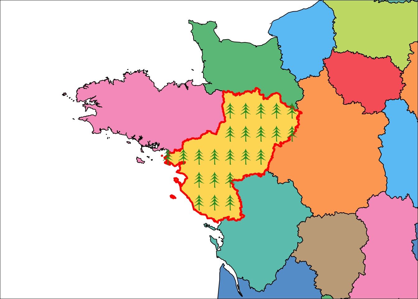

###Realize a grid point assuring icons not crossing lines

A problem with the previous code is that, depending on the locations sampled and on the size of emoji, icons may be out of the polygon. This arise because icons are centered on the position defined. To avoid this, we should sample locations in a polygon slightly smaller than the original. Function rgeos::gBuffer allows to calculate a buffer area around a spatial feature. Using a negative width on a SpatialPolygons creates a polygon with a smaller size (orange area on the figure below). The appropriate width helps avoid plotting icons out of the polygon.

# Realize a grid point assuring icons not crossing lines -----------------------
# icons half size
px_size <- 0.15
# Create a Buffer ith negative width to reduce polygon size
polBuf <- gBuffer(pol, width = -px_size)
# Sample in the buffer
grid.pt <- sp::spsample(polBuf, n = 25, type = "regular")

par(mai = c(0, 0, 0, 0))
# plot the entire map with restricted limits
plot(ext.pol, xaxs = "i", yaxs = "i", border = NA)
plot(fra.sp, col = scales::alpha(col.region, alpha = 0.7), add = TRUE)
# Highlight the selected polygon
plot(pol, border = "red", lwd = 3, add = TRUE)
# Show buffer area where no points
plot(polBuf, col = scales::alpha("red", 0.5) , border = NA, add = TRUE)
# Add emojifont instead of points
text(coordinates(grid.pt)[, 1], coordinates(grid.pt)[, 2],
     labels = emoji('evergreen_tree'), cex = 2, lwd = 3,
     col = 'forestgreen', family = 'OpenSansEmoji')
box()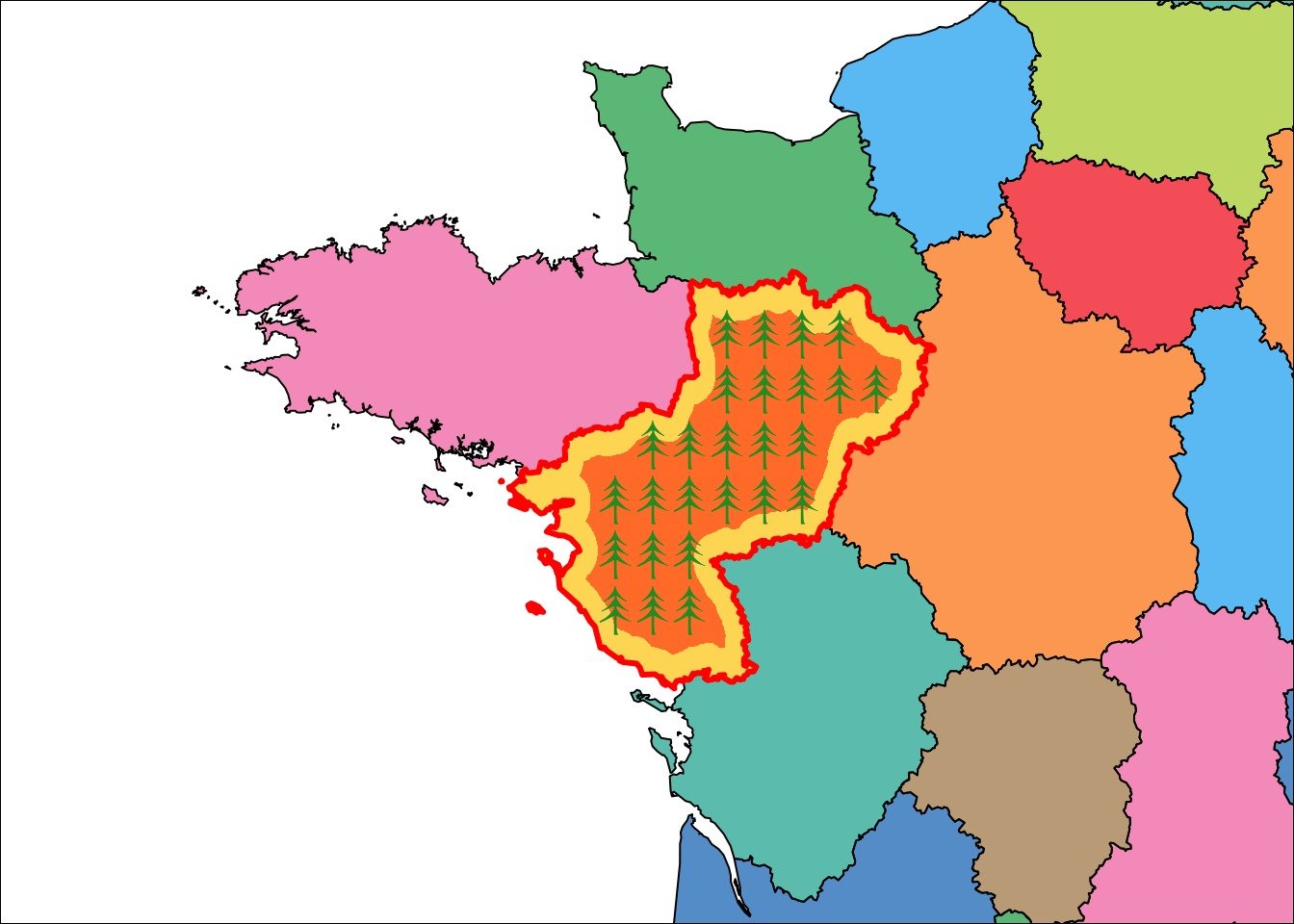

###Add your own image as a repeated pattern

Using emoji is an easy task, but you may want to use your own image. I used an other answer on stackoverflow to realize this with function graphics::rasterImage, coupled with the buffer polygon. Here I use an example with the R-logo so that you can reproduce the example, but any PNG image would work.

# Add your own image as a repeated pattern -------------------------------------
iconfile1 <- download.file('https://www.r-project.org/logo/Rlogo.png',
                           destfile = file.path(imgWD, 'icon1.png'), mode = 'wb')
icon1 <- png::readPNG(file.path(imgWD, 'icon1.png'))

# Define the desired size of the image
offset <- 0.1

par(mai = c(0, 0, 0, 0))
# plot the entire map with restricted limits
plot(ext.pol, xaxs = "i", yaxs = "i", border = NA)
plot(fra.sp, col = scales::alpha(col.region, alpha = 0.7), add = TRUE)
# Show buffer area where no points
plot(pol, border = "red", lwd = 3, add = TRUE)
# Plot all images at points locations
for (i in 1:length(grid.pt)) {
  graphics::rasterImage(
    icon1, 
    coordinates(grid.pt)[i, 1] - offset,
    coordinates(grid.pt)[i, 2] - offset,
    coordinates(grid.pt)[i, 1] + offset,
    coordinates(grid.pt)[i, 2] + offset
  )
}
box()

###Function to crop image within the limits of a polygon

Plotting with the buffer polygon requires to first calculate the size of your images in the spatial scale to be sure that images will not be plot out of the polygon area. You may want to avoid this calculation or you may want to avoid the white buffer area in your map. If your polygon is so small that the image do not fit entirely in, this may also be a problem. I thus created a function that give a transparent color to pixels of each images that are out of the polygon boudaries. To do so, I combined rasterImage and function mask of library raster, which work on Raster objects. I also made this function to work with ggplot2.

# Function to crop image within the limits of a polygon ----------------------

#' Plot your own image at a specific position cropped in a delimited polygon.
#' 
#' @param path path to PNG image to be added to the plot
#' @param offset vector of size 1 or 2. Size of the image in the scale of coordinates system of pol
#' @param offset.pc vector of size 1 or 2. Percent of the extent of the polygon.
#' @param pt coordinates where to plot the raster (x, y)
#' @param pol polygon to limit extent of the raster
#' @param type "normal" or "ggplot", matrix or tbl to be plotted
#' @param plot logical wether to plot (TRUE) or to return matrix/tbl for future plot (FALSE)

rasterImageCropPt <- function(path, offset, offset.pc, pt, pol,
                              type = "normal", plot = TRUE) {
  # Transform as raster (not Raster) to be plot by rasterImage
  r.png <- as.raster(png::readPNG(path))
  # Read as Raster to be cropped by polygon
  r <- raster(path, 1)
  # Calculate extent of the raster
  if (!missing(offset)) {
    # offset is image size
    offset <- 0.5 * offset
    if (length(offset) == 1) {offset <- rep(offset, 2)}
    xmin <- pt[1] - offset[1]
    xmax <- pt[1] + offset[1]
    ymin <- pt[2] - offset[2]
    ymax <- pt[2] + offset[2]
  }
  if (!missing(offset.pc)) {
    # offset is image size
    offset.pc <- 0.5 * offset.pc
    if (length(offset.pc) == 1) {offset.pc <- rep(offset.pc, 2)}
    xmin <- pt[1] - offset.pc[1]/100 * (xmax(pol) - xmin(pol))
    xmax <- pt[1] + offset.pc[1]/100 * (xmax(pol) - xmin(pol))
    ymin <- pt[2] - offset.pc[2]/100 * (ymax(pol) - ymin(pol))
    ymax <- pt[2] + offset.pc[2]/100 * (ymax(pol) - ymin(pol))
  }
  extent(r) <- c(xmin, xmax, ymin, ymax)
  projection(r) <- projection(pol)
  r.res <- mask(r, pol)
  
  # Add transparency to areas out of the polygon
  r.mat <- as.matrix(r.res)
  r.png[is.na(r.mat)] <- "#FFFFFF00"
  
  # Transform for ggplot
  if (type == "ggplot") {
    r.png <- data.frame(coordinates(r), value = c(t(as.matrix(r.png)))) %>% as.tbl()
  }
  
  if (plot) {
    if (type == "normal") {
      graphics::rasterImage(r.png, xmin, ymin, xmax, ymax)
    } else {
      return(geom_tile(data = r.png, aes(x, y), fill = r.png$value))
    } 
  } else {
    return(r.png)
  }
}

###Add your own image as repeated pattern within a polygon, cropped when needed

With my function, it is possible to plot our repeated image pattern without the use of the buffer. Images along borders get transparent pixels if they are out of the area. R-logo are bigger to better see what happens.

# Add your own image as repeated pattern in a polygon, cropped when needed -----
# Realise a point grid in a specific polygon, no buffer needed
grid.pt <- sp::spsample(pol, n = 15, type = "regular")

# Image size
offset <- 0.4

# plot the entire map with restricted limits
par(mai = c(0, 0, 0, 0))
# plot the entire map with restricted limits
plot(ext.pol, xaxs = "i", yaxs = "i", border = NA)
plot(fra.sp, col = scales::alpha(col.region, alpha = 0.7), add = TRUE)
# Plot images
for (i in 1:length(grid.pt)) {
  rasterImageCropPt(path = file.path(imgWD, 'icon1.png'), offset,
                    pt = coordinates(grid.pt)[i, ], 
                    pol = pol, type = "normal", plot = TRUE)  
}
box()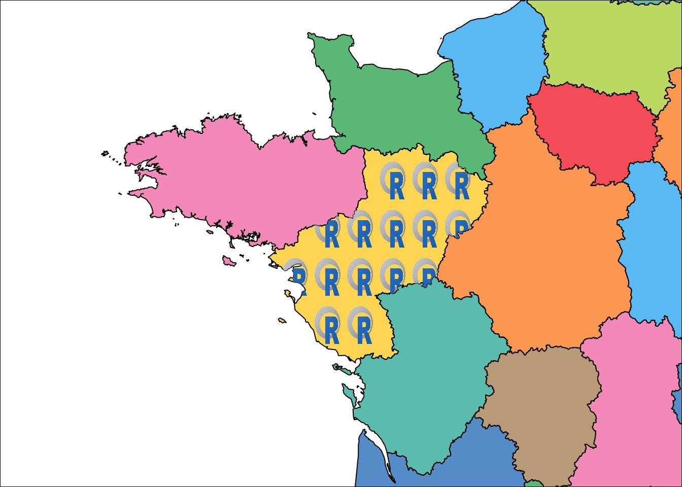

###Create a wallpaper image with repeated pattern

I must admit that function raster::mask used in my function makes it a little long to calculate, in particular because the image needs to be repeated for each point of the pattern. If you have a big polygon with image repeated many times, the image may be long to appear with the for-loop.

You may want to do it only once. For that, you can first create your own PNG image wallpaper with the repeated pattern (or any combination of images wanted). Here I create my wallpaper directly in R, but you can use any PNG image.

# Create a wallpaper image with repeated pattern -------------------------------
path.wp <- file.path(tmpImgWD, "figure-html", "wallpaper.png")

pol_square <- Polygon(coords = matrix(c(0,1,1,0,0,
                                        0,0,1,1,0), ncol = 2))
grid.wp <- sp::spsample(pol_square, n = 100, type = "regular")

offset <- 0.03

png(filename = path.wp, 
    width = 600, height = 600, unit = "px") 
par(mai = c(0.1,0.1,0.1,0.1), bg = "transparent", xpd = TRUE)
plot(grid.wp, col = "transparent")
for (i in 1:length(grid.wp)) {
  graphics::rasterImage(
    icon1, 
    coordinates(grid.wp)[i, 1] - offset,
    coordinates(grid.wp)[i, 2] - offset,
    coordinates(grid.wp)[i, 1] + offset,
    coordinates(grid.wp)[i, 2] + offset
  )
}
dev.off()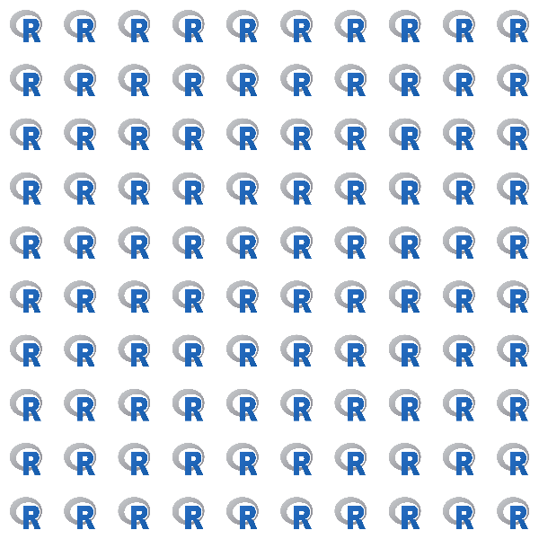

###Add your own wallpaper with repeated images in a polygon

Once your PNG image pattern wallpaper is created, you can use my function once to plot inside your polygon. While using parameter offset or, like here offset.pc, you make sure that your wallpaper covers 100% of your polygon and that images are not distorted.

# Add your own wallpaper with repeated images in a polygon ---------------------
ratio.pol <- (xmax(pol) - xmin(pol)) / (ymax(pol) - ymin(pol))

# plot the entire map with restricted limits
par(mai = c(0, 0, 0, 0))
# plot the entire map with restricted limits
plot(ext.pol, xaxs = "i", yaxs = "i", border = NA)
plot(fra.sp, col = scales::alpha(col.region, alpha = 0.7), add = TRUE)

# Add in the middle of the polygon
rasterImageCropPt(path = path.wp, offset.pc = c(100 * ratio.pol, 100),
                  pt = c(xmin(pol) + (xmax(pol) - xmin(pol))/2,
                         ymin(pol) + (ymax(pol) - ymin(pol))/2),
                  pol = pol, type = "normal", plot = TRUE)  
box()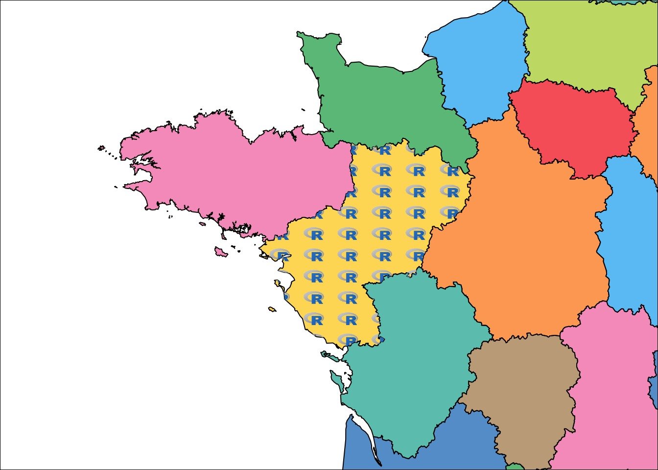

###Add your own wallpaper with repeated images in a polygon with ggplot ####Directly in the ggplot pipe

As I said earlier, my function may also be used in ggplot using type = ggplot. You can insert it directly in your piped ggplot syntax.

# Add your own wallpaper with repeated images in a polygon with ggplot ---------
# Direct ----
# Transform spatial data as `sf` objectas it is easier with ggplot
fra.sf <- sf::st_as_sf(fra.sp)

ggplot() +
  geom_sf(data = fra.sf,  aes(fill = NAME), col = "black") +
  scale_fill_manual(values = scales::alpha(col.region, alpha = 0.7),
                    breaks = fra.sp$NAME) +
  coord_sf(xlim = c(xmin(ext.pol), xmax(ext.pol)), 
           ylim = c(ymin(ext.pol), ymax(ext.pol)),
           expand = FALSE) +
  rasterImageCropPt(path = path.wp, offset.pc = c(100 * ratio.pol, 100),
                    pt = c(xmin(pol) + (xmax(pol) - xmin(pol))/2,
                           ymin(pol) + (ymax(pol) - ymin(pol))/2),
                    pol = pol, type = "ggplot", plot = TRUE) +
  guides(colour = FALSE, fill = FALSE)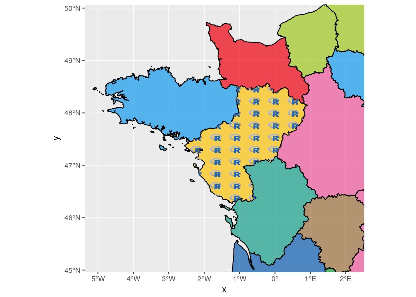

####Indirectly by creating the dataset to be plot with tiles

You can also run my function previous to the ggplot and retrieve the data.tbl necessary to add in your ggplot, using parameter add=FALSE. You can then plot it using geom_tiles as in my function. If you want to reduce the weight of the cropped image, you can also filter the transparent tiles before plotting. Here I also modified the offset.pc parameter to increase the size of R-logo images.

# Indirect ----
dataPNG <- rasterImageCropPt(
  path = path.wp,
  offset.pc = c(100 * ratio.pol, 100),
  pt = c(xmin(pol) + (xmax(pol) - xmin(pol))/2,
         ymin(pol) + (ymax(pol) - ymin(pol))/2),
  pol = pol, type = "ggplot", plot = FALSE)
# You can filter transparent tiles (out of the area)
dataPNG.filter <- filter(dataPNG, value != "#FFFFFF00")


ggplot() +
  geom_sf(data = fra.sf,  aes(fill = NAME), col = "black") +
    scale_fill_manual(values = scales::alpha(col.region, alpha = 0.7),
                      breaks = fra.sp$NAME) +
    coord_sf(xlim = c(xmin(ext.pol), xmax(ext.pol)), 
                  ylim = c(ymin(ext.pol), ymax(ext.pol)),
             expand = FALSE) +
  geom_tile(data = dataPNG.filter, aes(x, y), fill = dataPNG.filter$value) +
  guides(colour = FALSE, fill = FALSE)

Create wallpaper for symbology with emoji

Instead of using the R-logo wallpaper, we create one with emoji. To avoid a bad resolution of symbols when we stretch the image to the SpatialPolygons size, we can create a wallpaper adapted to the size using the width/height ratio. I also changed the regular sampling in the spatial polygon so that geographic coordinates of points are shifted with option type = hexagonal.

# Create a wallpaper image with repeated emoji and polygon dimensions ----
path.wp <- file.path(extraWD, "wallpaperEmoji.png")
ratio.pol <- (xmax(pol) - xmin(pol)) / (ymax(pol) - ymin(pol))

pol_square <- Polygon(coords = 
                        matrix(c(0,ratio.pol,ratio.pol,0,0,
                                 0,0,1,1,0),
                               ncol = 2))
grid.wp <- sp::spsample(pol_square, n = 100, type = "hexagonal")

png(filename = path.wp, 
    width = 300 * ratio.pol, height = 300, unit = "px") 
par(mai = c(0.1,0.1,0.1,0.1), bg = "transparent", xpd = TRUE)
plot(grid.wp, col = "transparent")

text(coordinates(grid.wp)[, 1], coordinates(grid.wp)[, 2],
     labels = emoji('evergreen_tree'), cex = 3, lwd = 4,
     col = 'forestgreen', family = 'OpenSansEmoji')
dev.off()

We insert it in a ggplot2 figure with library sf.

dataPNG <- rasterImageCropPt(
  path = path.wp,
  offset.pc = c(100, 100),
  pt = c(xmin(pol) + (xmax(pol) - xmin(pol))/2,
         ymin(pol) + (ymax(pol) - ymin(pol))/2),
  pol = pol, type = "ggplot", plot = FALSE)
# You can filter transparent tiles (out of the area)
dataPNG.filter <- filter(dataPNG, value != "#FFFFFF00")

ggplot() +
  geom_sf(data = fra.sf,  aes(fill = NAME), col = "black") +
    scale_fill_manual(values = scales::alpha(col.region, alpha = 0.7),
                      breaks = fra.sp$NAME) +
    coord_sf(xlim = c(xmin(ext.pol), xmax(ext.pol)), 
                  ylim = c(ymin(ext.pol), ymax(ext.pol)),
             expand = FALSE) +
  geom_tile(data = dataPNG.filter, aes(x, y), fill = dataPNG.filter$value) +
  guides(colour = FALSE, fill = FALSE)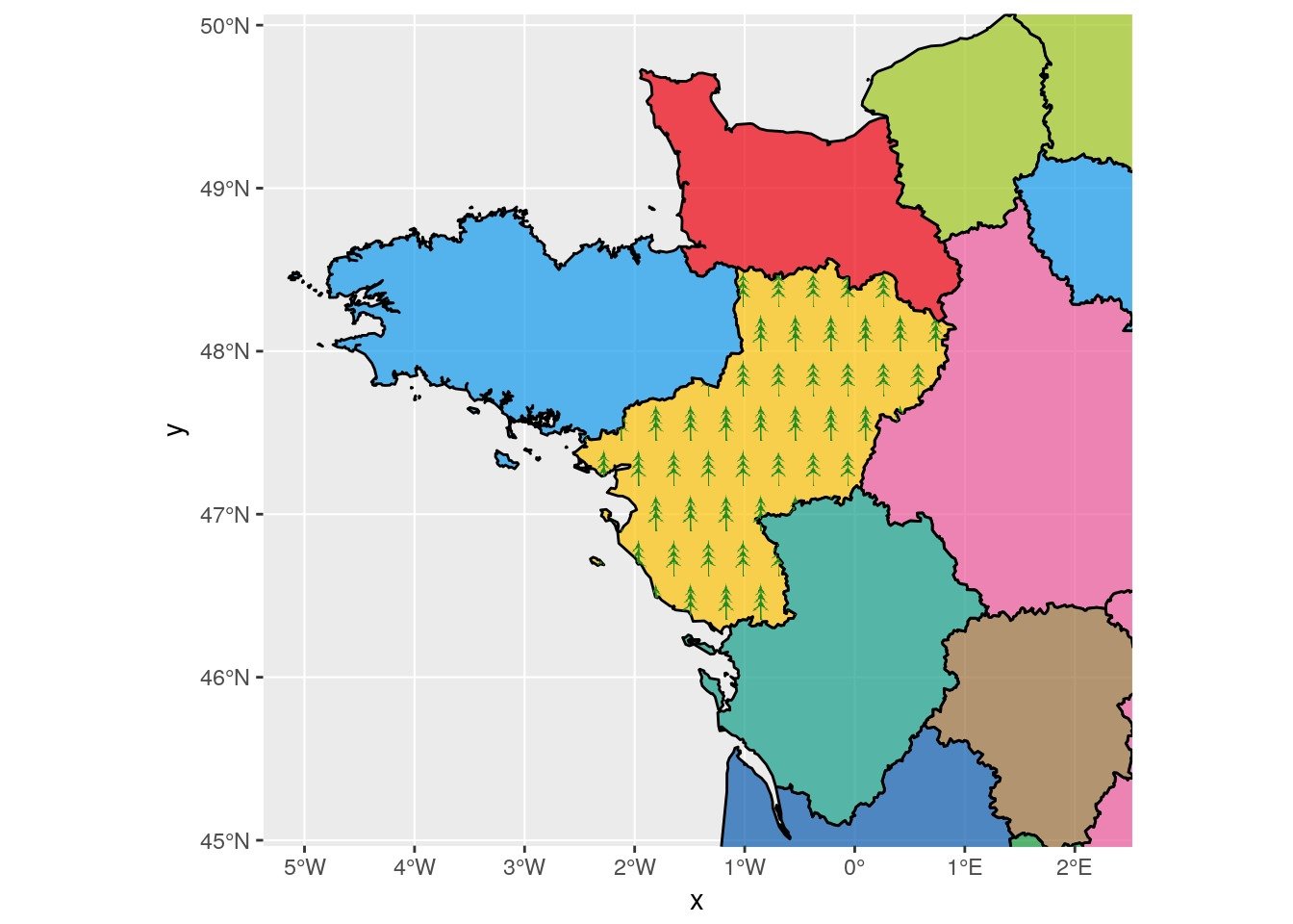

The complete code to plot a specific image in a delimited polygon as repeated pattern on a map is on my github