Afficher un motif d’images répétées dans un polygone
De la symbologie en cartographie avec R
Une question sur stackoverflow demandait comment dessiner des arbres dans un polygone pour représenter une forêt sur une carte. J’ai d’abord pensé à afficher des émoticônes d’arbres sur une grille régulière au sein du polygone. La librairie sp permet justement de faire ce type d’échantillonnage régulier dans un SpatialPolygon. J’ai aussi pensé à comment afficher ma propre image sur cette grille régulière, à l’aide de la fonction rasterImage. Ici, nous irons un peu plus loin dans la symbologie SIG pour les polygones avec Rstats, notamment avec une fonction maison, un peu plus avancée de rasterImage.
Le script complet est ici.
Des données
Définissons d’abord un SpatialPolygonDataFrame avec lequel travailler. Définissons aussi un polygone dans lequel dessiner la forêt.
# Load global map
fra.sp.orig <- getData('GADM', country = 'FRA', level = 1, path = extraWD)
fra.sp <- gSimplify(fra.sp.orig, tol = 0.005) %>%
  SpatialPolygonsDataFrame(data = data.frame(NAME = fra.sp.orig$NAME_1))

# Select polygon in which adding symbols
pol <- fra.sp[which(fra.sp$NAME == "Pays de la Loire"),]

# Define extent for figures
e <- extend(extent(pol), c(2.75, 1.6, 1.3, 1.5))
ext.pol <- SpatialPolygons(list(Polygons(list(Polygon(
  rbind(c(e@xmin, e@ymin), c(e@xmin, e@ymax),
        c(e@xmax, e@ymax), c(e@xmax, e@ymin),
        c(e@xmin, e@ymin)))), ID = 1)))
proj4string(ext.pol) <- proj4string(fra.sp)

# Define colors fixed for some regions
col.n <- c(9,1,4,2,3,6,4,5,5,6,7,6,7,10,7,3,9,8,7,9,7,1)
col.region <- yarrr::piratepal("basel")[col.n]
Dessiner une grille régulière de points avec des émoticônes dans un polygone spécifique
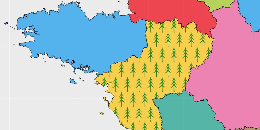
Il est possible d’échantillonner des points sur une grille régulière dans un polygone « spatial » avec la fonction sp::spsample. On peut ensuite afficher sur ces coordonnées, une émoticône en utilisant la librairie emoji par exemple.
# Create a point grid in a specific polygon -----------------------------------
grid.pt <- sp::spsample(pol, n = 25, type = "regular")

par(mai = c(0, 0, 0, 0))
# plot the entire map with restricted limits
plot(ext.pol, xaxs = "i", yaxs = "i", border = NA)
plot(fra.sp, col = scales::alpha(col.region, alpha = 0.7), add = TRUE)
# Highlight the selected polygon
plot(pol, border = "red", lwd = 3, add = TRUE)
# Normal points
points(grid.pt, pch = 20, col = "blue", cex = 0.1)
# Add emojifont instead of points
text(coordinates(grid.pt)[, 1], coordinates(grid.pt)[, 2],
     labels = emoji('evergreen_tree'), cex = 2, lwd = 3,
     col = 'forestgreen', family = 'OpenSansEmoji')
box()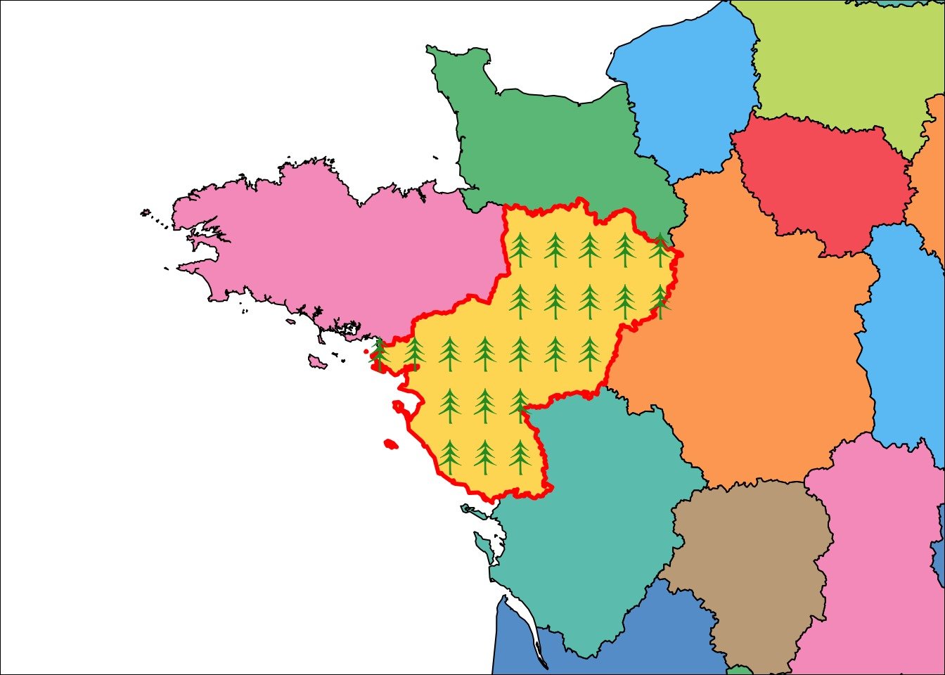
Réaliser une grille de point en s’assurant que les icônes ne sortent pas du polygone
Un problème avec le code précédent c’est que, selon la position des points sélectionnés et la taille de l’émoticône choisie, les icônes peuvent se trouver en dehors du polygone. C’est parce que l’icône est centrée sur la coordonnées. Pour éviter cela, on peut échantillonner les positions dans un polygone légèrement plus petit que l’original. La function rgeos::gBuffer permet de calculer une zone tampon autour d’un objet géographique. En utilisant une distance négative sur un objet de classe SpatialPolygon, il est possible de créer un polygone plus petit (zone rouge sur la figure suivante). La distance appropriée permet d’éviter l’affichage des émoticônes en dehors du polygone.
# Realize a grid point assuring icons not crossing lines -----------------------
# icons half size
px_size <- 0.15
# Create a Buffer ith negative width to reduce polygon size
polBuf <- gBuffer(pol, width = -px_size)
# Sample in the buffer
grid.pt <- sp::spsample(polBuf, n = 25, type = "regular")

par(mai = c(0, 0, 0, 0))
# plot the entire map with restricted limits
plot(ext.pol, xaxs = "i", yaxs = "i", border = NA)
plot(fra.sp, col = scales::alpha(col.region, alpha = 0.7), add = TRUE)
# Highlight the selected polygon
plot(pol, border = "red", lwd = 3, add = TRUE)
# Show buffer area where no points
plot(polBuf, col = scales::alpha("red", 0.5) , border = NA, add = TRUE)
# Add emojifont instead of points
text(coordinates(grid.pt)[, 1], coordinates(grid.pt)[, 2],
     labels = emoji('evergreen_tree'), cex = 2, lwd = 3,
     col = 'forestgreen', family = 'OpenSansEmoji')
box()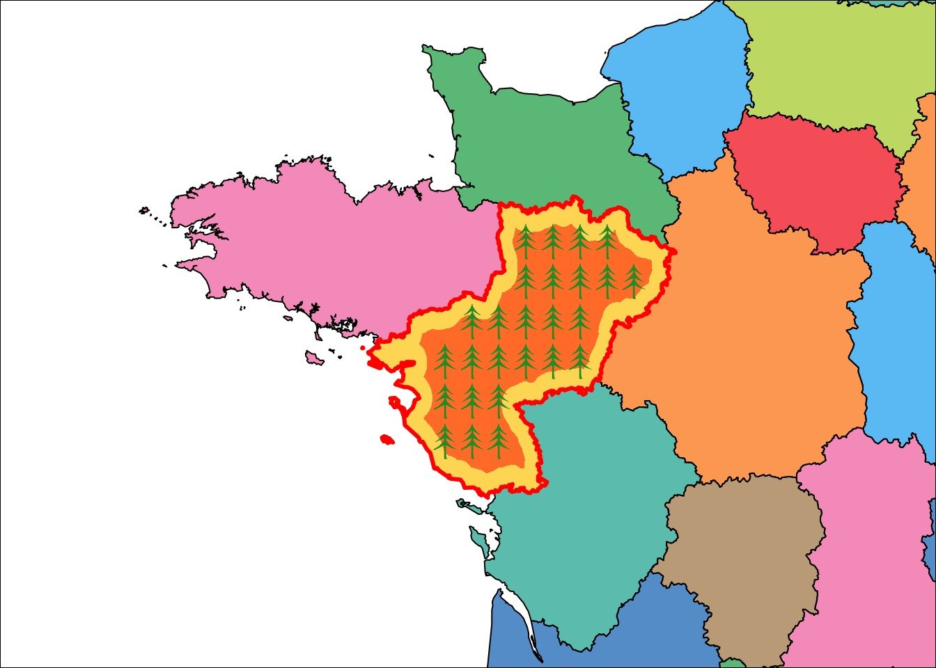
Ajouter votre propre image comme un motif répété
Utiliser une émoticône est assez facile, mais vous pourriez vouloir utiliser votre propre image. J’ai utilisé une autre réponse sur stackoverflow pour permettre d’utiliser votre propre image comme motif, en utilisant la fonction graphics::rasterImage et toujours la zone tampon. Ici, j’utilise le logo R pour que l’exemple soit reproductible mais n’importe quelle image PNG fera l’affaire.
# Add your own image as a repeated pattern -------------------------------------
iconfile1 <- download.file('https://www.r-project.org/logo/Rlogo.png',
                           destfile = file.path(extraWD, figure-html', 'icon1.png'), mode = 'wb')
icon1 <- png::readPNG(file.path(extraWD, 'icon1.png'))

# Define the desired size of the image
offset <- 0.1

par(mai = c(0, 0, 0, 0))
# plot the entire map with restricted limits
plot(ext.pol, xaxs = "i", yaxs = "i", border = NA)
plot(fra.sp, col = scales::alpha(col.region, alpha = 0.7), add = TRUE)
# Show buffer area where no points
plot(pol, border = "red", lwd = 3, add = TRUE)
# Plot all images at points locations
for (i in 1:length(grid.pt)) {
  graphics::rasterImage(
    icon1,
    coordinates(grid.pt)[i, 1] - offset,
    coordinates(grid.pt)[i, 2] - offset,
    coordinates(grid.pt)[i, 1] + offset,
    coordinates(grid.pt)[i, 2] + offset
  )
}
box()
Une fonction pour restreindre les images à la zone définie par le polygone
Créer l’image à l’aide de la zone tampon nécessite d’abord de calculer la taille de votre image dans l’échelle spatiale de votre carte, de façon à vous assurer qu’elles ne sortiront pas du polygone. Vous pourriez avoir envie d’éviter ce calcul. Vous pourriez aussi vouloir qu’il n’y ait pas de zone blanche autour de vos images dans le polygone. Par ailleurs, si votre polygone est si petit que votre image ne peut y tenir entièrement, vous êtes bloqués. J’ai donc créé une fonction qui donne une couleur transparente aux pixels de chaque image se trouvant en dehors du polygone. Pour cela, j’ai combiné la function rasterImage avec la fonction mask de la librairie raster fonctionnant sur les objets de type Raster. J’ai aussi fait en sorte que cette fonction marche avec ggplot2.
# Function to crop image within the limits of a polygon ----------------------

#' Plot your own image at a specific position cropped in a delimited polygon.
#'
#' @param path path to PNG image to be added to the plot
#' @param offset vector of size 1 or 2. Size of the image in the scale of coordinates system of pol
#' @param offset.pc vector of size 1 or 2. Percent of the extent of the polygon.
#' @param pt coordinates where to plot the raster (x, y)
#' @param pol polygon to limit extent of the raster
#' @param type "normal" or "ggplot", matrix or tbl to be plotted
#' @param plot logical wether to plot (TRUE) or to return matrix/tbl for future plot (FALSE)

rasterImageCropPt <- function(path, offset, offset.pc, pt, pol,
                              type = "normal", plot = TRUE) {
  # Transform as raster (not Raster) to be plot by rasterImage
  r.png <- as.raster(png::readPNG(path))
  # Read as Raster to be cropped by polygon
  r <- raster(path, 1)
  # Calculate extent of the raster
  if (!missing(offset)) {
    # offset is image size
    offset <- 0.5 * offset
    if (length(offset) == 1) {offset <- rep(offset, 2)}
    xmin <- pt[1] - offset[1]
    xmax <- pt[1] + offset[1]
    ymin <- pt[2] - offset[2]
    ymax <- pt[2] + offset[2]
  }
  if (!missing(offset.pc)) {
    # offset is image size
    offset.pc <- 0.5 * offset.pc
    if (length(offset.pc) == 1) {offset.pc <- rep(offset.pc, 2)}
    xmin <- pt[1] - offset.pc[1]/100 * (xmax(pol) - xmin(pol))
    xmax <- pt[1] + offset.pc[1]/100 * (xmax(pol) - xmin(pol))
    ymin <- pt[2] - offset.pc[2]/100 * (ymax(pol) - ymin(pol))
    ymax <- pt[2] + offset.pc[2]/100 * (ymax(pol) - ymin(pol))
  }
  extent(r) <- c(xmin, xmax, ymin, ymax)
  projection(r) <- projection(pol)
  r.res <- mask(r, pol)

  # Add transparency to areas out of the polygon
  r.mat <- as.matrix(r.res)
  r.png[is.na(r.mat)] <- "#FFFFFF00"

  # Transform for ggplot
  if (type == "ggplot") {
    r.png <- data.frame(coordinates(r), value = c(t(as.matrix(r.png)))) %>% as.tbl()
  }

  if (plot) {
    if (type == "normal") {
      graphics::rasterImage(r.png, xmin, ymin, xmax, ymax)
    } else {
      return(geom_tile(data = r.png, aes(x, y), fill = r.png$value))
    }
  } else {
    return(r.png)
  }
}
Ajouter une image, tronquée si nécessaire, comme motif répété dans un polygone
Avec ma fonction, il est possible de créer votre motif sans avoir besoin de la zone tampon. Les images le long des bords du polygone qui dépassent un peu, se retrouvent avec quelques pixels transparents. J’ai agrandit les images pour mieux voir la découpe.
# Add your own image as repeated pattern in a polygon, cropped when needed -----
# Realise a point grid in a specific polygon, no buffer needed
grid.pt <- sp::spsample(pol, n = 15, type = "regular")

# Image size
offset <- 0.4

# plot the entire map with restricted limits
par(mai = c(0, 0, 0, 0))
# plot the entire map with restricted limits
plot(ext.pol, xaxs = "i", yaxs = "i", border = NA)
plot(fra.sp, col = scales::alpha(col.region, alpha = 0.7), add = TRUE)
# Plot images
for (i in 1:length(grid.pt)) {
  rasterImageCropPt(path = file.path(tmpImgWD, 'icon1.png'), offset,
                    pt = coordinates(grid.pt)[i, ],
                    pol = pol, type = "normal", plot = TRUE)
}
box()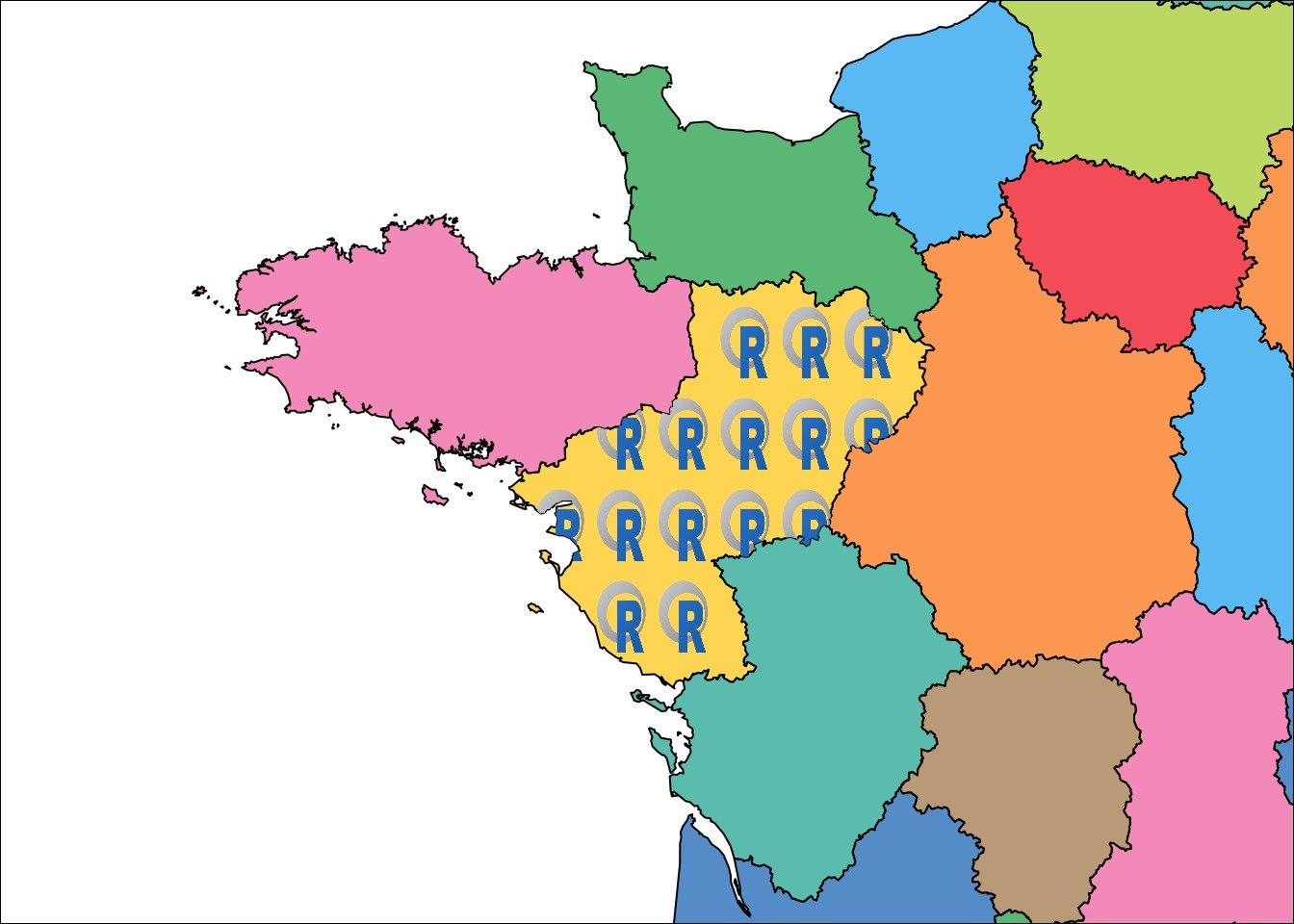
Créer un papier peint avec votre image comme motif repété
Je dois admettre que la fonction raster::mask utilisée dans ma fonction rend le calcul parfois un peu long. En particulier parce que la fonction doit être utilisée pour chacune des images affichées dans le motif avec la boucle for. Si vous avez un gros polygone avec de nombreuses répétitions de votre image, l’affichage va être très long…
Vous pourriez donc avoir envie de faire l’opération une seule fois. Pour cela, je vous encourage à créer votre papier peint, votre motif de symbologie au format PNG avant toute opération. Il contiendra votre motif répété d’images ou n’importe quelle combinaison d’images. Ici, je crée mon papier peint directement dans R pour que vous puissiez reproduire le code, mais vous pouvez utiliser n’importe quelle image PNG.
# Create a wallpaper image with repeated pattern -------------------------------
path.wp <- file.path(tmpImgWD, "figure-html", "wallpaper.png")

pol_square <- Polygon(coords = matrix(c(0,1,1,0,0,
                                        0,0,1,1,0), ncol = 2))
grid.wp <- sp::spsample(pol_square, n = 100, type = "regular")

offset <- 0.03

png(filename = path.wp,
    width = 600, height = 600, unit = "px")
par(mai = c(0.1,0.1,0.1,0.1), bg = "transparent", xpd = TRUE)
plot(grid.wp, col = "transparent")
for (i in 1:length(grid.wp)) {
  graphics::rasterImage(
    icon1,
    coordinates(grid.wp)[i, 1] - offset,
    coordinates(grid.wp)[i, 2] - offset,
    coordinates(grid.wp)[i, 1] + offset,
    coordinates(grid.wp)[i, 2] + offset
  )
}
dev.off()
Ajouter votre papier avec des images répété à l’intérieur d’un polygone
Une fois votre papier peint créé, vous pouvez utiliser ma fonction directement. En choisissant les bonnes dimensions avec l’une des options offset ou offset.pc comme ici, vous vous assurez que votre papier couvre au moins 100% de la taille du polygone et que les motifs ne sont pas déformés.
# Add your own wallpaper with repeated images in a polygon ---------------------
ratio.pol <- (xmax(pol) - xmin(pol)) / (ymax(pol) - ymin(pol))

# plot the entire map with restricted limits
par(mai = c(0, 0, 0, 0))
# plot the entire map with restricted limits
plot(ext.pol, xaxs = "i", yaxs = "i", border = NA)
plot(fra.sp, col = scales::alpha(col.region, alpha = 0.7), add = TRUE)

# Add in the middle of the polygon
rasterImageCropPt(path = path.wp, offset.pc = c(100 * ratio.pol, 100),
                  pt = c(xmin(pol) + (xmax(pol) - xmin(pol))/2,
                         ymin(pol) + (ymax(pol) - ymin(pol))/2),
                  pol = pol, type = "normal", plot = TRUE)
box()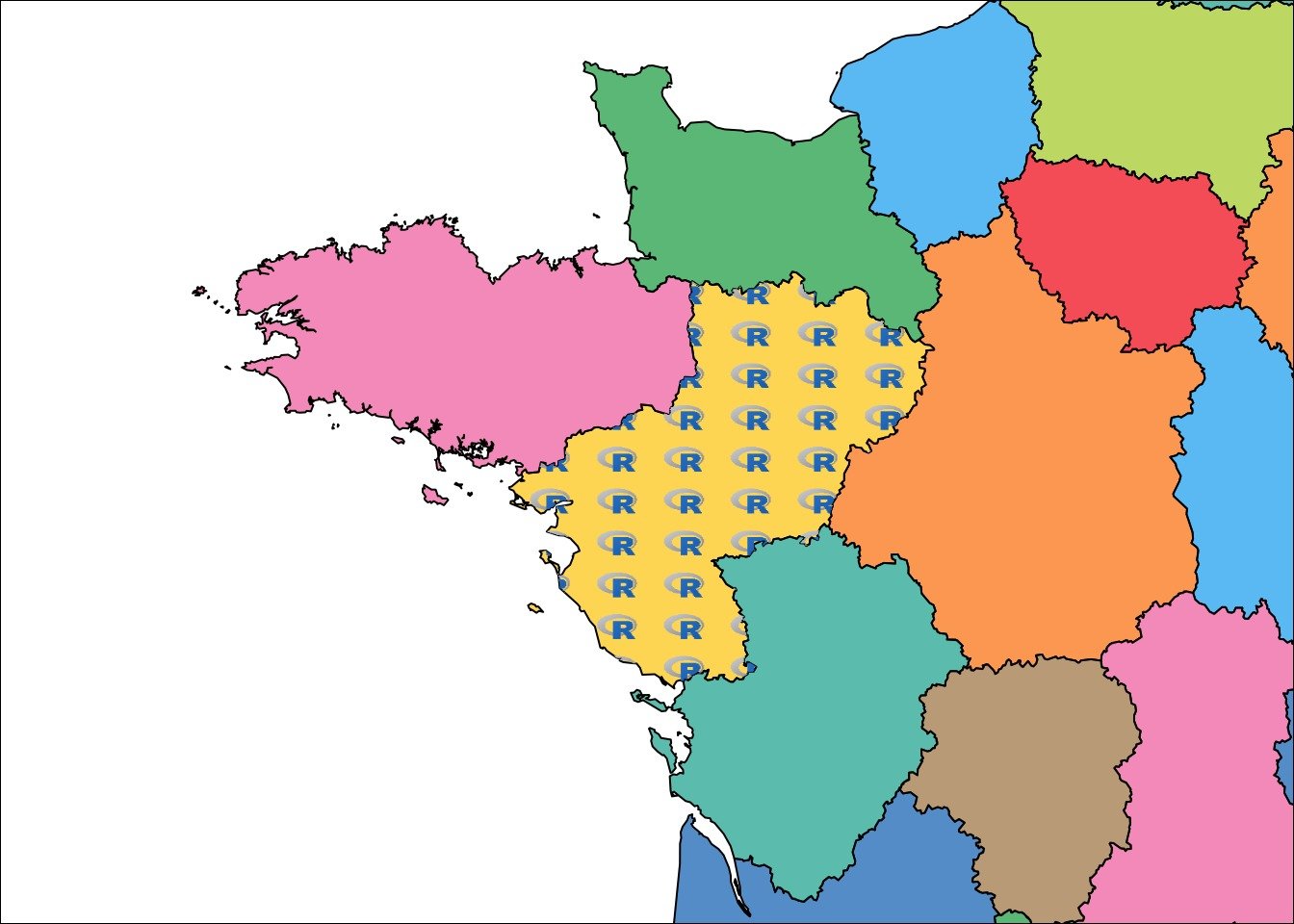
Ajouter votre papier avec des images répété à l’intérieur d’un polygone avec ggplot
Directement dans un pipe ggplot2
Comme écrit plus haut, ma fonction peut aussi être utilisée avec ggplot2 avec l’option type = ggplot. Vous pouvez l’insérer directement dans votre syntaxe ggplot.
# Add your own wallpaper with repeated images in a polygon with ggplot ---------
# Direct ----
# Transform spatial data as `sf` objectas it is easier with ggplot
fra.sf <- sf::st_as_sf(fra.sp)

ggplot() +
  geom_sf(data = fra.sf,  aes(fill = NAME), col = "black") +
  scale_fill_manual(values = scales::alpha(col.region, alpha = 0.7),
                    breaks = fra.sp$NAME) +
  coord_sf(xlim = c(xmin(ext.pol), xmax(ext.pol)),
           ylim = c(ymin(ext.pol), ymax(ext.pol)),
           expand = FALSE) +
  rasterImageCropPt(path = path.wp, offset.pc = c(100 * ratio.pol, 100),
                    pt = c(xmin(pol) + (xmax(pol) - xmin(pol))/2,
                           ymin(pol) + (ymax(pol) - ymin(pol))/2),
                    pol = pol, type = "ggplot", plot = TRUE) +
  guides(colour = FALSE, fill = FALSE)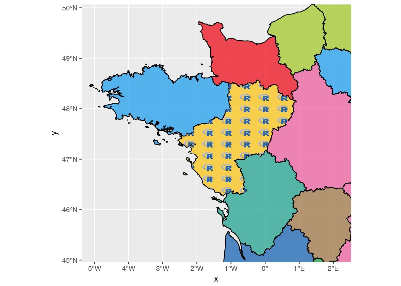
Indirectement en créant un jeu de données utilisable par ggplot avec des tuiles
Vous pouvez aussi utiliser ma fonction avant de créer votre ggplot pour récupérer uniquement la table de données au format data.tbl qui pourra être utilisée dans ggplot, grâce à l’option plot = FALSE. Vous pourrez ensuite utiliser la fonction geom_tiles comme au sein de ma fonction. Si vous voulez réduire le poids de l’image découpée, vous pouvez aussi filtrer les pixels transparent avant de faire votre figure. Ici, j’ai aussi modifié l’option offset.pc pour affcher les logos R de mon papier peint en plus gros.
# Indirect ----
dataPNG <- rasterImageCropPt(
  path = path.wp,
  offset.pc = c(100 * ratio.pol, 100),
  pt = c(xmin(pol) + (xmax(pol) - xmin(pol))/2,
         ymin(pol) + (ymax(pol) - ymin(pol))/2),
  pol = pol, type = "ggplot", plot = FALSE)
# You can filter transparent tiles (out of the area)
dataPNG.filter <- filter(dataPNG, value != "#FFFFFF00")


ggplot() +
  geom_sf(data = fra.sf,  aes(fill = NAME), col = "black") +
    scale_fill_manual(values = scales::alpha(col.region, alpha = 0.7),
                      breaks = fra.sp$NAME) +
    coord_sf(xlim = c(xmin(ext.pol), xmax(ext.pol)),
                  ylim = c(ymin(ext.pol), ymax(ext.pol)),
             expand = FALSE) +
  geom_tile(data = dataPNG.filter, aes(x, y), fill = dataPNG.filter$value) +
  guides(colour = FALSE, fill = FALSE)
Créer un papier peint pour une symbology avec des émoticônes
Plutôt que d’utiliser la papier peint avec des images du logo R, on peut en créer un avec nos emoji. Pour éviter une mauvaise résolution des symboles lorsqu’on étire le papier peint à la taille du polygone, on peut créer un papier adapté sachant le ratio hauteur/largeur du polygone spatial. J’ai ausi changé l’échantillonnage régulier dans le polygone spatial de telle sorte que les coordonnées géographiques des points soient décalées avec l’option type = "hexagonal".
# Create a wallpaper image with repeated emoji and polygon dimensions ----
path.wp <- file.path(extraWD, "wallpaperEmoji.png")
ratio.pol <- (xmax(pol) - xmin(pol)) / (ymax(pol) - ymin(pol))

pol_square <- Polygon(coords =
                        matrix(c(0,ratio.pol,ratio.pol,0,0,
                                 0,0,1,1,0),
                               ncol = 2))
grid.wp <- sp::spsample(pol_square, n = 100, type = "hexagonal")

png(filename = path.wp,
    width = 300 * ratio.pol, height = 300, unit = "px")
par(mai = c(0.1,0.1,0.1,0.1), bg = "transparent", xpd = TRUE)
plot(grid.wp, col = "transparent")

text(coordinates(grid.wp)[, 1], coordinates(grid.wp)[, 2],
     labels = emoji('evergreen_tree'), cex = 3, lwd = 4,
     col = 'forestgreen', family = 'OpenSansEmoji')
dev.off()
On l’insère dans notre figure ggplot et librairie sf.
dataPNG <- rasterImageCropPt(
  path = path.wp,
  offset.pc = c(100, 100),
  pt = c(xmin(pol) + (xmax(pol) - xmin(pol))/2,
         ymin(pol) + (ymax(pol) - ymin(pol))/2),
  pol = pol, type = "ggplot", plot = FALSE)
# You can filter transparent tiles (out of the area)
dataPNG.filter <- filter(dataPNG, value != "#FFFFFF00")

ggplot() +
  geom_sf(data = fra.sf,  aes(fill = NAME), col = "black") +
    scale_fill_manual(values = scales::alpha(col.region, alpha = 0.7),
                      breaks = fra.sp$NAME) +
    coord_sf(xlim = c(xmin(ext.pol), xmax(ext.pol)),
                  ylim = c(ymin(ext.pol), ymax(ext.pol)),
             expand = FALSE) +
  geom_tile(data = dataPNG.filter, aes(x, y), fill = dataPNG.filter$value) +
  guides(colour = FALSE, fill = FALSE)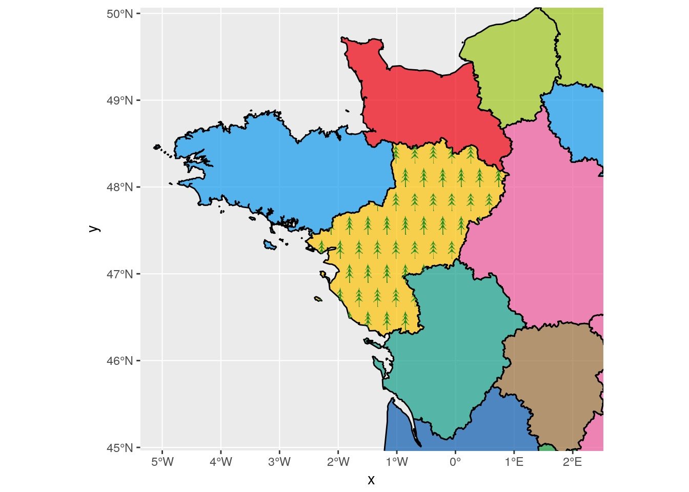
Citation :
Merci de citer ce travail avec :
Rochette Sébastien. (2017, avr.. 09). "Dessiner un motif d’images répétées sur une carte dans un polygone". Retrieved from https://statnmap.com/fr/2017-04-09-dessiner-motif-images-repetees-sur-carte-dans-polygone/.
Citation BibTex :
@misc{Roche2017Dessi,
    author = {Rochette Sébastien},
    title = {Dessiner un motif d’images répétées sur une carte dans un polygone},
    url = {https://statnmap.com/fr/2017-04-09-dessiner-motif-images-repetees-sur-carte-dans-polygone/},
    year = {2017}
  }