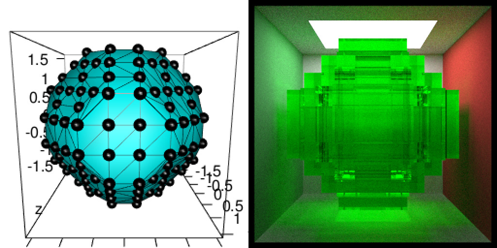
People like to show 3D images in their presentations because it usually impresses the audience. Does it really ? I do not care ! I am just looking for an opportunity to play with some 3D images…
This blog post is a detailed version of some 3D images shown during my presentation “Everything but maps with spatial tools” at SatRday Paris.
Rayshade 3D objects
I use to play with mesh3d objects using {rgl}. In a previous post, I already showed how to transform a 3dmesh into a 2D spatial raster object so that it can fit in {rayshader}. Indeed, {rayshader} and {rayrender} use 2D matrices to render 3D objects and I wanted to know how this would be possible to use 3D objects to be rayshaded directly. However, I do not want to build a new package for that. Tyler Morgan is doing a great job, I want to use what already exists. Using {rayshader} thus requires to transform a triangular 3D mesh into a rectangular 2D matrix to be able to render a 3D rectangular rayshaded form. With {rayrender}, this is a little more challenging. I needed to think my triangular 3D mesh as a voxelised 3D image. Yes, I like to think in a rectangular way…
Note that the functions presented in details in this blog post are all included in my package {mesh2ray} on Github so that you can transform your mesh3d objects in a rectangular way for {raster}, {rayshader} or {rayrender}.
# Packages
library(raster)
library(dplyr)
library(Rvcg)
library(rgl)
library(rayshader)
library(rayrender)
# remotes::install_github("statnmap/mesh2ray")
library(mesh2ray)
library(magick)
# Directories
# extraWD <- tmpImgWD <- ""
Steps of the method from mesh3d to {rayshader}
Images below show the complete procedure on a small mesh with a low resolution:
- If needed, cut the 3d mesh with
Morpho::cutMeshPlane() - Project the mesh over a 2D raster with
mesh2ray::mesh_to_raster() - Transform the mesh as a matrix for {rayshader} with
mesh2ray::stack_to_ray() - Plot your matrix using {rayshader}
# Create simple mesh
simple_mesh_orig <- Rvcg::vcgIcosahedron()

# 1. Cut it with a plane with {Morpho}
v1 <- c(0, 0, -0.5)
v2 <- c(1, 0, -0.5)
v3 <- c(0, 1, -0.5)
simple_mesh <- Morpho::cutMeshPlane(simple_mesh_orig, v1, v2, v3)

# _plot3d
plot3d(simple_mesh, col = "cyan")
aspect3d(1, 1, 0.2)
plot3d(simple_mesh, type = "wire", add = TRUE)
plot3d(t(simple_mesh$vb), type = "s", radius = 0.1, add = TRUE)
view3d(theta = 20, phi = -40, zoom = 0.5, fov = 80)
# _snapshot
rgl.snapshot(filename = file.path(extraWD, "rayshader-simple-1-mesh.png"))
rgl::rgl.close()

# 2. Project on raster
simple_r <- mesh2ray::mesh_to_raster(simple_mesh, res = 26)
png(filename = file.path(extraWD, "rayshader-simple-2-raster.png"))
plot(simple_r)
dev.off()

# 3. raster to matrix
simple_ray <- mesh2ray::stack_to_ray(simple_r)

# 4. Rayshade matrix
zscale <- 0.4
ambmat <- ambient_shade(simple_ray$elevation, zscale = zscale)
raymat <- ray_shade(simple_ray$elevation, zscale = zscale, lambert = TRUE,
                    sunangle = 300)

ray_image <- simple_ray$elevation %>%
  sphere_shade(texture = "unicorn") %>%
  add_shadow(raymat, max_darken = 0.1) %>%
  add_shadow(ambmat, max_darken = 0.5)

# _plot 3d
ray_image %>%
  plot_3d(simple_ray$elevation, zscale = zscale, windowsize = c(1000, 1000),
          soliddepth = -max(simple_ray$elevation, na.rm = TRUE)/zscale,
          theta = -30, phi = 50, zoom = 0.7, fov = 20
  )

# _snapshot
rgl.snapshot(filename = file.path(extraWD, "rayshader-simple-3-ray3d.png"))
rgl::rgl.close()

# Image montage
img_frames <- list.files(extraWD, pattern = "rayshader-simple", full.names = TRUE)
image_append(image_scale(image_read(img_frames), "400"))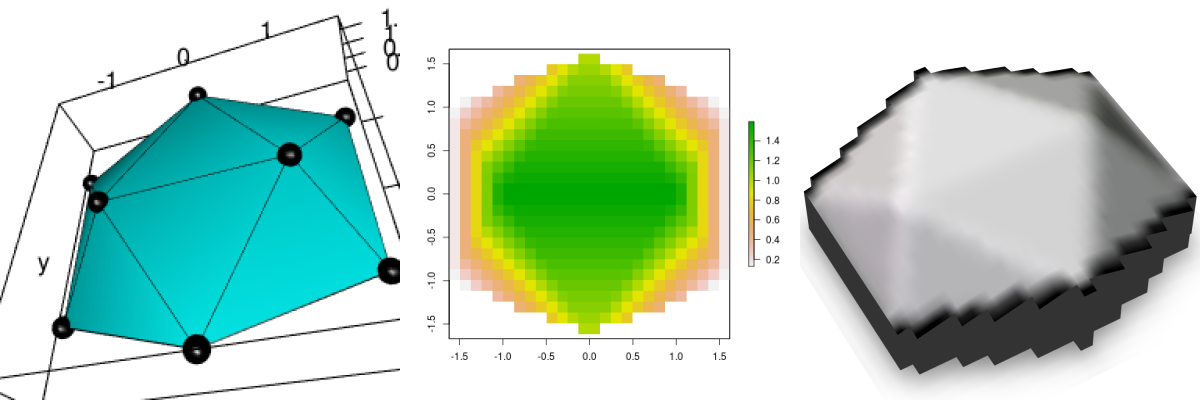
Figure 1: Low resolution rayshading. a. mesh3d, b. rasterized mesh, c. rayshaded rasterized mesh
Read 3D human face data
This time, I will not play with a plant meristem, but with a 3D mesh of a human face that is included in {Rvcg}, a powerful R-package providing mesh manipulation routines from VCGLIB.
data(humface)

# 1. Cut it with a plane with {Morpho}
v1 <- c(0, 0, -0.5)
v2 <- c(1, 0, -0.5)
v3 <- c(0, 1, -0.5)
hum_mesh <- Morpho::cutMeshPlane(humface, v1, v2, v3)

try(rgl.close(), silent = TRUE)
plot3d(hum_mesh, col = "cyan")
aspect3d("iso")
# Change view
view3d(theta = 20, phi = -20, zoom = 0.5)
rgl.snapshot(filename = file.path(tmpImgWD, "figure-html", "readhuman.png"))
rgl::rgl.close()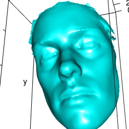
Render a mesh3d with {rayshader}
Transform a mesh3d as raster with {geometry}
The 3D human face can be projected in 2D. We can project it over a raster in the plane x/y. In the post with the 3D meristem, I used an inverse distance interpolation to estimate the height (z) of each cell of the projection raster. This calculation was quite heavy and I have hardly been able to use it on the human face mesh because it has a too high number of vertices (points). I tried different things with tools of my knowledge from {raster} package notably, but this was not enough. At least, I was able to produce something for my presentation “Everything but maps with spatial tools” at SatRday Paris on a low resolution version of the human face.
But I was not totally satisfied. I briefly discussed this on Twitter with Michael Sumner (mdsumner) who also like to play with 3D data and maps. A few hours later, he gave me a link to a script with a solution using geometry::tsearch. I enjoy so much how nice, friendly and welcoming is the R community !
Let’s build an empty raster of size 150*150, having the same x/y extent as our 3d face. The mesh3d object is a triangular mesh. In 2D, rach cell center of the empty raster falls in one of the triangles of the mesh. Using tsearch, you can find in which triangle of the mesh it falls. The function also returns the distance from the three angles of the triangle. With this information, you can interpolate linearly the z coordinates using a weighted mean (by the distance) of z of the three points of the triangle.
Note that this function is named mesh_to_raster() in my Github package {mesh2ray}
# If the orientation of the mesh please you,
# you can directly extract the xy vertices of the mesh triangles
# as a projection of the mesh on x/y
myMesh <- hum_mesh
triangle_xy <- t(myMesh$vb[1:2, ])
## Build a target raster with extent of the mesh
hum_mesh_r <- raster(extent(triangle_xy), nrows = 150, ncols = 150)
hum_mesh_r <- setValues(hum_mesh_r, NA_real_)
# Extract x/y coordinates of the raster
raster_xy <- sp::coordinates(hum_mesh_r)
## the magic barycentric index, the interpolation engine for the target grid vertices
## and where they fall in each triangle relative to triangle vertices
pid0 <- geometry::tsearch(x = triangle_xy[,1], y = triangle_xy[,2],
                          t = t(myMesh$it),
                          xi = raster_xy[,1], yi = raster_xy[, 2],
                          bary = TRUE)

# Determine raster cell center that really fall in a triangle of the mesh
ok <- !is.na(pid0$idx)
# Calculate linear interpolation of the z value using distances to vertices
hum_mesh_r[ok] <- colSums(matrix(myMesh$vb[3, myMesh$it[, pid0$idx[ok]]], nrow = 3) * t(pid0$p)[, ok])
# Plot the output raster
plot(hum_mesh_r)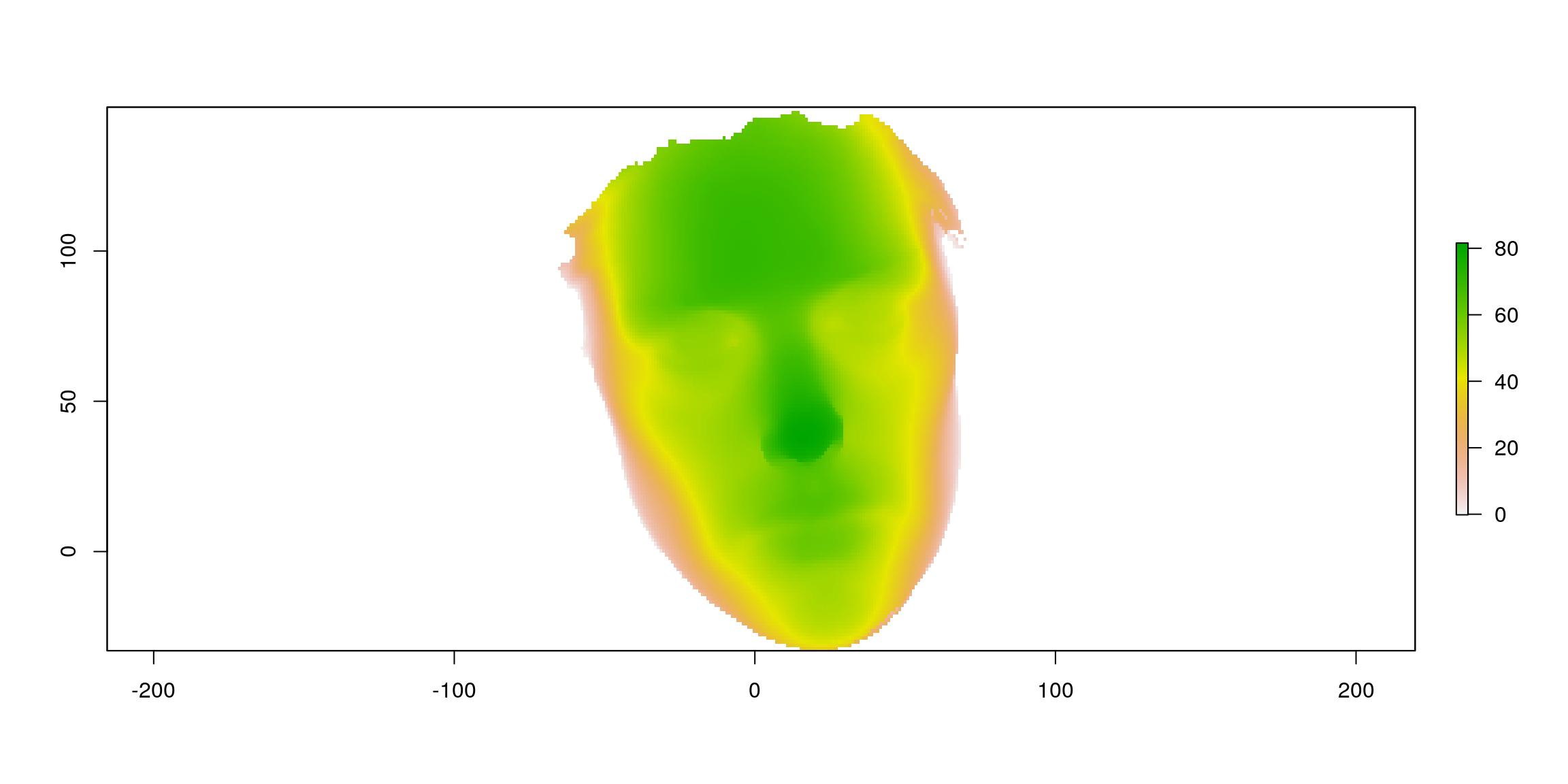
Render the resulting raster using {rayshader}
That is easy to transform a raster to a matrix as used by {rayshader}, you simply need to transpose a as.matrix().
datamat <- t(as.matrix(hum_mesh_r))
# Rayshade raster
zscale <- 0.1
ambmat <- ambient_shade(datamat, zscale = zscale)
raymat <- ray_shade(datamat, zscale = zscale, lambert = TRUE,
                    sunangle = 45)

ray_image <- datamat %>%
  sphere_shade(texture = "unicorn") %>%
  add_shadow(raymat, max_darken = 0.1) %>%
  add_shadow(ambmat, max_darken = 0.5)

plot_map(ray_image)
If you want to overlay an image that has nothing to do with your raster, this may be a little tricky. In package {mesh2ray}, you can use function stack_to_ray() to resample an image to the dimension of the raster and get the matrix needed.
By the way, a {rayshader} output would not be a proper {rayshader} output without a gif…
r_img <- stack(file.path(extraWD, "ThinkR_logo_500px.png"))
hum_mesh_img <- stack_to_ray(hum_mesh_r, r_img)

# Rayshade raster
zscale <- 0.25
ambmat <- ambient_shade(hum_mesh_img$elevation, zscale = zscale)
raymat <- ray_shade(hum_mesh_img$elevation, zscale = zscale, lambert = TRUE)

ray_image_overlay <- hum_mesh_img$elevation %>%
  sphere_shade(texture = "imhof4") %>%
  add_overlay(hum_mesh_img$overlay, alphalayer = 0.99) %>% # Note overlay
  add_shadow(raymat, max_darken = 0.01) %>%
  add_shadow(ambmat, max_darken = 0.5) # %>%
# add_water(watermap, color = "#57B6FF")

# transform as gif
path_gif <- file.path(extraWD, "face.gif")
if (!file.exists(path_gif)) {
  # Add some movement
  th <- seq(-50, 50, length.out = 20)
  ph <- seq(80, 90, length.out = 20)
  move <- data.frame(theta = c(th, rev(th)), phi = c(ph, rev(ph)))

  n_frames <- nrow(move)
  dir.create(file.path(extraWD, "face_gif"), showWarnings = FALSE)
  img_frames <- file.path(
    extraWD, "face_gif",
    paste0("face", formatC(seq_len(n_frames), width = 3, flag = "0"), ".png"))

  # create all frames
  for (i in seq_len(n_frames)) {
    ray_image_overlay %>%
      plot_3d(hum_mesh_img$elevation, zscale = zscale, windowsize = c(1000, 1000),
              soliddepth = -max(hum_mesh_img$elevation, na.rm = TRUE)/zscale,
              theta = move$theta[i], phi = move$phi[i], zoom = 0.30, fov = 20
      )

    rgl::snapshot3d(img_frames[i])
    rgl::clear3d()
  }
  rgl::rgl.close()

  magick::image_write_gif(magick::image_read(img_frames),
                          path = path_gif,
                          delay = 6/n_frames)
}
file.copy(file.path(extraWD, "face.gif"),
          file.path(glue("../../static{StaticImgWD}/face.gif")),
          overwrite = TRUE)
Render a mesh3d with {rayrender}
{rayrender} can draw cubes using position of its center and dimensions in x, y and z. To render a triangular mesh, I imagined it as a voxelized image. It is the same as in 2D dimension when I transformed the mesh into a 2D regular grid, except this will be a 3D regular grid.
{Rvcg} has powerful tools to work with big mesh. For instance, function vcgUniformRemesh() resamples a mesh uniformly. This means that the new points of the regular mesh can be used as my cube centers. I then just have to calculte the distance between each cube center in x, y and z to build the cubes.
Steps of the method from mesh3d to {rayrender}
Images below show the complete procedure on a small mesh with a low resolution:
- Uniformely re-sampled the 3d mesh with
Rvcg::vcgUniformRemesh - Extract information of the uniform mesh with
mesh2ray::mesh_to_cubes(that includesvcgUniformRemesh) - Add cubes to the scene with
mesh2ray::add_cubes_to_scene - Plot the scene using {rayrender}
# Create simple mesh
simple_mesh <- Rvcg::vcgIcosahedron()

# _plot3d
plot3d(simple_mesh, col = "cyan")
aspect3d("iso")
plot3d(simple_mesh, type = "wire", add = TRUE)
plot3d(t(simple_mesh$vb), type = "s", radius = 0.1, add = TRUE)
view3d(theta = 0, phi = 10, zoom = 0.6, fov = 80)
# _snapshot
rgl.snapshot(filename = file.path(extraWD, "rayrender-simple-1-mesh.png"))
rgl::rgl.close()

# 1. Uniformely resample mesh
# _vcgUniformRemesh is included in mesh_to_cubes()
simple_resample <- vcgUniformRemesh(simple_mesh, voxelSize = 0.5, multiSample = TRUE,
                                discretize = TRUE)

plot3d(simple_resample, col = "cyan")
aspect3d("iso")
plot3d(simple_resample, type = "wire", add = TRUE)
plot3d(t(simple_resample$vb), type = "s", radius = 0.1, add = TRUE)
view3d(theta = 0, phi = 10, zoom = 0.6, fov = 80)
# _snapshot
rgl.snapshot(filename = file.path(extraWD, "rayrender-simple-2-regularmesh.png"))
rgl::rgl.close()

# 2. Calculate cube positions in a specific scene
# _vcgUniformRemesh is included in mesh_to_cubes()
simple_cubes <- mesh2ray::mesh_to_cubes(simple_mesh, voxelSize = 0.5, scene_dim = c(80, 475))

# 3. Draw with rayrender
# _scene
scene <- generate_cornell(lightintensity = 10)
# _add cubes on scene
scene <- mesh2ray::add_cubes_to_scene(scene, cubes = simple_cubes,
                                      material = dielectric(color = "green"))
# _draw scene /!\ long calculation /!\
if (!file.exists(file.path(extraWD, "rayrender-simple-3-scene.png"))) {
  options(cores = 4)
  render_scene(scene, lookfrom = c(278, 278, -800) ,
               lookat = c(278, 278, 0), fov = 40, ambient_light = FALSE,
               samples = 500, parallel = TRUE, clamp_value = 5,
               filename =  file.path(extraWD, "rayrender-simple-3-scene.png"))
}

# Image montage
img_frames <- list.files(extraWD, pattern = "rayrender-simple", full.names = TRUE)
image_append(image_scale(image_read(img_frames), "400"))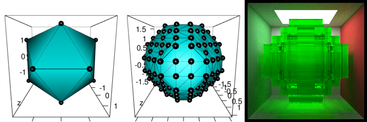
Figure 2: Low resolution rayrendering. a. mesh3d, b. regularly sampled mesh, c. rayrendered regularly sampled mesh
Apply voxelisation on the human face and defines colours
The steps are the same than the small example above. We are using a higher resolution to get a final form much closer to the original.
However, I wanted to add some colours to some of the cubes and to do so, I did some manual drawing on 2D plots. After a few spatial points and polygons manipulations using {sf}, I can have a colored version of the face in 2D.
# voxelisation
data(humface)
human_cubes <- mesh2ray::mesh_to_cubes(humface, voxelSize = 0.5, scene_dim = c(20, 535))

# Define colours areas manually
polygon_contours_file <- file.path(extraWD, "polygon_contours.rds")
if (!file.exists(polygon_contours_file)) {
  # Manually draw polygons
  plot(human_cubes$cube_center$x, human_cubes$cube_center$y, pch = 20, cex = 0.5)

  eye1 <- raster::drawPoly(col = "blue")
  eye2 <- raster::drawPoly(col = "blue")
  mouth <- raster::drawPoly(col = "red")
  front <- raster::drawPoly(col = "green")

  polygon_contours <- list(eye1 = eye1, eye2 = eye2, mouth = mouth, front = front)
  # Transform as sf polygon
  polygon_contours_sf <- polygon_contours %>%
  purrr::map2(names(polygon_contours),
              ~sf::st_as_sf(.x) %>% mutate(name = .y)) %>%
  do.call("rbind", .)

  readr::write_rds(polygon_contours_sf, polygon_contours_file)
} else {
  polygon_contours_sf <- readr::read_rds(polygon_contours_file)
}

# Transform cubes as sf for intersection with contours
human_colours <- human_cubes$cube_center %>%
  sf::st_as_sf(coords = c("x", "y"), remove = FALSE) %>%
  sf::st_join(polygon_contours_sf) %>%
  mutate(colours = case_when(
    name %in% c("eye1", "eye2") ~ "blue",
    name == "mouth" ~ "red",
    name == "front" ~ "ivory",
    TRUE ~ "grey"
  )) %>%
  as_tibble()

# Explore the 3D points and color
plot3d(t(human_cubes$mesh_resample$vb), type = "s", radius = 1,
       col = human_colours$colours)
aspect3d("iso")
view3d(theta = 0, phi = 10, zoom = 0.6, fov = 80)
# _snapshot
rgl.snapshot(filename = file.path(tmpImgWD, "figure-html/humcolours.png"))
rgl::rgl.close()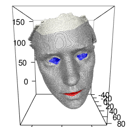
Define material for each cube
I can create a tibble containing a material for each of the cubes to draw.
# All types of cubes
colours_cubes <- bind_rows(
  lambertian(color = "ivory"),
  dielectric(color = "#2E7BE6"),
  dielectric(color = "#2E7BE6"),
  dielectric(color = "#DB3B3B"),
  dielectric()
) %>%
  mutate(name = c(NA, "eye1", "eye2", "mouth", "front"))

# Join with table of colours
human_materials <- dplyr::select(human_colours, name) %>%
  left_join(colours_cubes, by = "name") %>%
dplyr::select(-name)human_materials## # A tibble: 245,975 x 12
## type properties checkercolor noise noisephase noiseintensity noisecolor
## <chr> <list> <list> <dbl> <dbl> <dbl> <list>
## 1 lamb… <dbl [3]> <dbl [2]> 0 0 10 <dbl [3]>
## 2 lamb… <dbl [3]> <dbl [2]> 0 0 10 <dbl [3]>
## 3 lamb… <dbl [3]> <dbl [2]> 0 0 10 <dbl [3]>
## 4 lamb… <dbl [3]> <dbl [2]> 0 0 10 <dbl [3]>
## 5 lamb… <dbl [3]> <dbl [2]> 0 0 10 <dbl [3]>
## 6 lamb… <dbl [3]> <dbl [2]> 0 0 10 <dbl [3]>
## 7 lamb… <dbl [3]> <dbl [2]> 0 0 10 <dbl [3]>
## 8 lamb… <dbl [3]> <dbl [2]> 0 0 10 <dbl [3]>
## 9 lamb… <dbl [3]> <dbl [2]> 0 0 10 <dbl [3]>
## 10 lamb… <dbl [3]> <dbl [2]> 0 0 10 <dbl [3]>
## # … with 245,965 more rows, and 5 more variables: image <list>,
## # lightintensity <lgl>, fog <lgl>, fogdensity <dbl>, implicit_sample <lgl>Draw the complete scene
The voxelised human_cubes object needs to be added to the empty scene using mesh2ray::add_cubes_to_scene with the tibble of materials created. Drawing the scene requires some time… Be patient… You can parallelise the calculations to reduce time.
# 3. Draw with rayrender
if (!file.exists(file.path(extraWD, "rayrender-human-scene.png"))) {
  # _scene
  scene <- generate_cornell(lightintensity = 20)
  # _add cubes on scene with material data.frame /!\ A little long /!\
  scene <- mesh2ray::add_cubes_to_scene(scene, cubes = human_cubes,
                                        material = human_materials)

  # _draw scene /!\ long calculation /!\
  options(cores = 4)
  render_scene(scene, width = 600, height = 600,
               lookfrom = c(278, 278, -800) ,
               lookat = c(278, 278, 0), fov = 40, ambient_light = FALSE,
               samples = 500, parallel = TRUE, clamp_value = 5,
               filename =  file.path(tmpImgWD, "figure-html/rayrender-human-scene.png"))
}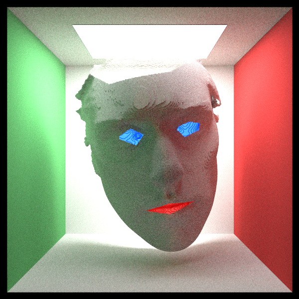
Tada ! Now, it’s your turn. Although this two {rayshader} and {rayrender} packages are young, there are already many possibilities. I am sure there will be a lot of great inventions around them. And always remember to take some time to have fun ! R is also here for that !
Resources
Noteworthy packages used here are:
- {rayshader} and {rayrender} for ray tracing. Have a look at Tyler Morgan blog here.
- {Morpho} and {Rvcg} for 3d mesh manipulation. Have a look at Stefan Schlager blog here.
- {mesh2ray} that I share on github
The complete list of packages is the following:
attachment::att_from_rmd("2019-04-02-mesh3d-rayshader-and-rayrender.Rmd")## [1] "raster" "dplyr" "Rvcg" "rgl" "rayshader"
## [6] "rayrender" "mesh2ray" "magick" "readr" "attachment"As always, the complete R script of this article can be found on my Blog Tips Github repository.
Citation:
For attribution, please cite this work as:
Rochette Sébastien. (2019, Apr. 10). "Render mesh3d objects with rayshader and rayrender". Retrieved from https://statnmap.com/2019-04-02-mesh3d-rayshader-and-rayrender/.
BibTex citation:
@misc{Roche2019Rende,
    author = {Rochette Sébastien},
    title = {Render mesh3d objects with rayshader and rayrender},
    url = {https://statnmap.com/2019-04-02-mesh3d-rayshader-and-rayrender/},
    year = {2019}
  }

