Les gens aiment montrer des images 3D dans leurs présentations parce qu’elles font généralement un petit effet “wahou”. Enfin, est-ce vraiment le cas ? A vrai dire, peu m’importe ! Je cherche juste une opportunité de jouer avec des images 3D…
Cet article de blog est une version détaillée de quelques images 3D de ma présentation “Everything but maps with spatial tools” à SatRday Paris.
Rayshade des ojets 3D
J’ai l’habitude de jouer avec des objets mesh3d en utilisant {rgl}. Dans un article précédent, j’ai déjà montré comment transformer un 3dmesh en un objet raster spatial 2D pour qu’il puisse tenir dans {rayshader}. En effet, {rayshader} et {rayrender} utilisent des matrices 2D pour rendre des objets 3D et je voulais savoir comment il serait possible d’utiliser des objets 3D pour être rayshadés directement. Mais, je n’ai pas l’intention de construire un nouveau paquet pour cela. Tyler Morgan fait du bon boulot, je vais utiliser au mieux l’existant. L’utilisation de {rayshader} nécessite donc de transformer un maillage 3D triangulaire en une matrice 2D rectangulaire pour pouvoir rendre une forme 3D rectangulaire rayshadée. Avec {rayrender}, c’est un peu plus difficile. J’avais besoin de penser mon maillage 3D triangulaire comme une image 3D voxélisée. Oui, j’aime bien penser de manière rectangulaire…
Notez que les fonctions présentées en détail dans ce post sont toutes incluses dans mon package {mesh2ray} sur Github qui vous serviria à transformer vos objets mesh3d de manière rectangulaire pour {raster}, {rayshader} ou {rayrender}.
# Packages
library(raster)
library(dplyr)
library(Rvcg)
library(rgl)
library(rayshader)
library(rayrender)
# remotes::install_github("statnmap/mesh2ray")
library(mesh2ray)
library(magick)
# Directories
# extraWD <- tmpImgWD <- ""
Étapes de la méthode des mesh3d vers {rayshader}
Les images ci-dessous montrent la procédure complète sur un petit mesh3d avec une faible résolution :
- Si nécessaire, coupez le mesh3d avec
Morpho::cutMeshPlane(). - Projeter le mesh3d sur un raster 2D avec
mesh2ray::mesh_to_raster(). - Transformez le mesh3d en matrice pour {rayshader} avec
mesh2ray::stack_to_ray(). - Tracez votre matrice avec {rayshader}.
# Create simple mesh
simple_mesh_orig <- Rvcg::vcgIcosahedron()

# 1. Cut it with a plane with {Morpho}
v1 <- c(0, 0, -0.5)
v2 <- c(1, 0, -0.5)
v3 <- c(0, 1, -0.5)
simple_mesh <- Morpho::cutMeshPlane(simple_mesh_orig, v1, v2, v3)

# _plot3d
plot3d(simple_mesh, col = "cyan")
aspect3d(1, 1, 0.2)
plot3d(simple_mesh, type = "wire", add = TRUE)
plot3d(t(simple_mesh$vb), type = "s", radius = 0.1, add = TRUE)
view3d(theta = 20, phi = -40, zoom = 0.5, fov = 80)
# _snapshot
rgl.snapshot(filename = file.path(extraWD, "rayshader-simple-1-mesh.png"))
rgl::rgl.close()

# 2. Project on raster
simple_r <- mesh2ray::mesh_to_raster(simple_mesh, res = 26)
png(filename = file.path(extraWD, "rayshader-simple-2-raster.png"))
plot(simple_r)
dev.off()

# 3. raster to matrix
simple_ray <- mesh2ray::stack_to_ray(simple_r)

# 4. Rayshade matrix
zscale <- 0.4
ambmat <- ambient_shade(simple_ray$elevation, zscale = zscale)
raymat <- ray_shade(simple_ray$elevation, zscale = zscale, lambert = TRUE,
                    sunangle = 300)

ray_image <- simple_ray$elevation %>%
  sphere_shade(texture = "unicorn") %>%
  add_shadow(raymat, max_darken = 0.1) %>%
  add_shadow(ambmat, max_darken = 0.5)

# _plot 3d
ray_image %>%
  plot_3d(simple_ray$elevation, zscale = zscale, windowsize = c(1000, 1000),
          soliddepth = -max(simple_ray$elevation, na.rm = TRUE)/zscale,
          theta = -30, phi = 50, zoom = 0.7, fov = 20
  )

# _snapshot
rgl.snapshot(filename = file.path(extraWD, "rayshader-simple-3-ray3d.png"))
rgl::rgl.close()

# Image montage
img_frames <- list.files(extraWD, pattern = "rayshader-simple", full.names = TRUE)
image_append(image_scale(image_read(img_frames), "400"))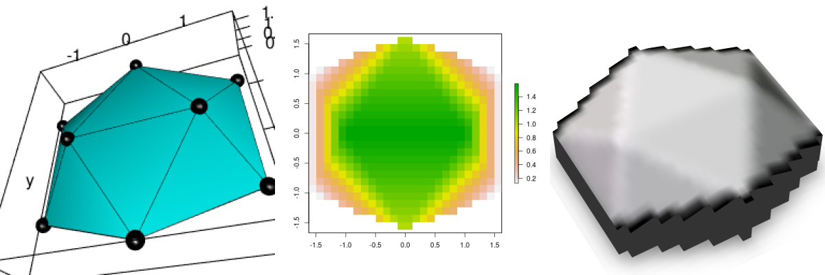
Figure 1: Low resolution rayshading. a. mesh3d, b. rasterized mesh, c. rayshaded rasterized mesh
Lire les données d’une image 3D de face humaine
Cette fois, je ne joue pas avec un méristème de plante, mais avec un mesh3d d’une face humaine qui est incluse dans {Rvcg}, un package R puissant avec des routines de manipulation de mesh à l’aide de VCGLIB.
data(humface)

# 1. Cut it with a plane with {Morpho}
v1 <- c(0, 0, -0.5)
v2 <- c(1, 0, -0.5)
v3 <- c(0, 1, -0.5)
hum_mesh <- Morpho::cutMeshPlane(humface, v1, v2, v3)

try(rgl.close(), silent = TRUE)
plot3d(hum_mesh, col = "cyan")
aspect3d("iso")
# Change view
view3d(theta = 20, phi = -20, zoom = 0.5)
rgl.snapshot(filename = file.path(tmpImgWD, "figure-html", "readhuman.png"))
rgl::rgl.close()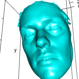
Afficher un mesh3d avec {rayshader}
Transformer un mesh3d en raster avec {geometry}
Le visage humain 3D peut être projeté en 2D. On peut le projeter sur un raster sur le plan x/y. Dans l’article avec le méristeme 3D, j’ai utilisé une interpolation en distance inverse pour estimer la hauteur (z) de chaque cellule du raster de projection. Ce calcul était assez lourd et j’ai à peine pu l’utiliser sur le mesh du visage car il a un trop grand nombre de sommets (points). J’ai essayé différentes choses avec les outils que je connais dans le package {raster} notamment, mais ce n’était pas suffisant. Au moins, j’ai pu produire quelque chose pour ma présentation “Everything but maps with spatial tools” à SatRday Paris sur une version basse résolution du visage humain.
Je n’étais pas totalement satisfait. J’en ai brièvement discuté sur Twitter avec Michael Sumner (mdsumner) qui aime aussi jouer avec les données 3D et les cartes. Quelques heures plus tard, il m’a envoyé un lien vers un script avec une solution utilisant geometry::tsearch. J’aime trop cette communauté R sympathique, amicale et accueillante !
Construisons un raster vide de taille 150*150, ayant les mêmes dimensions x/y que notre visage 3d. L’objet mesh3d a un maillage triangulaire. À plat, chaque centre de cellule du raster vide tombe dans un des triangles du raster. En utilisant tsearch, on peut trouver dans quel triangle du mesh, le centre du raster se trouve. La fonction renvoie aussi la distance depuis les trois angles du triangle. Avec cette information, on peut interpoler linéairement les coordonnées z en utilisant une moyenne pondérée (par la distance) du z des trois points du triangle.
Notez que cette fonction est nommée mesh_to_raster() dans mon paquet Github {mesh2ray}.
# If the orientation of the mesh please you,
# you can directly extract the xy vertices of the mesh triangles
# as a projection of the mesh on x/y
myMesh <- hum_mesh
triangle_xy <- t(myMesh$vb[1:2, ])
## Build a target raster with extent of the mesh
hum_mesh_r <- raster(extent(triangle_xy), nrows = 150, ncols = 150)
hum_mesh_r <- setValues(hum_mesh_r, NA_real_)
# Extract x/y coordinates of the raster
raster_xy <- sp::coordinates(hum_mesh_r)
## the magic barycentric index, the interpolation engine for the target grid vertices
## and where they fall in each triangle relative to triangle vertices
pid0 <- geometry::tsearch(x = triangle_xy[,1], y = triangle_xy[,2],
                          t = t(myMesh$it),
                          xi = raster_xy[,1], yi = raster_xy[, 2],
                          bary = TRUE)

# Determine raster cell center that really fall in a triangle of the mesh
ok <- !is.na(pid0$idx)
# Calculate linear interpolation of the z value using distances to vertices
hum_mesh_r[ok] <- colSums(matrix(myMesh$vb[3, myMesh$it[, pid0$idx[ok]]], nrow = 3) * t(pid0$p)[, ok])
# Plot the output raster
plot(hum_mesh_r)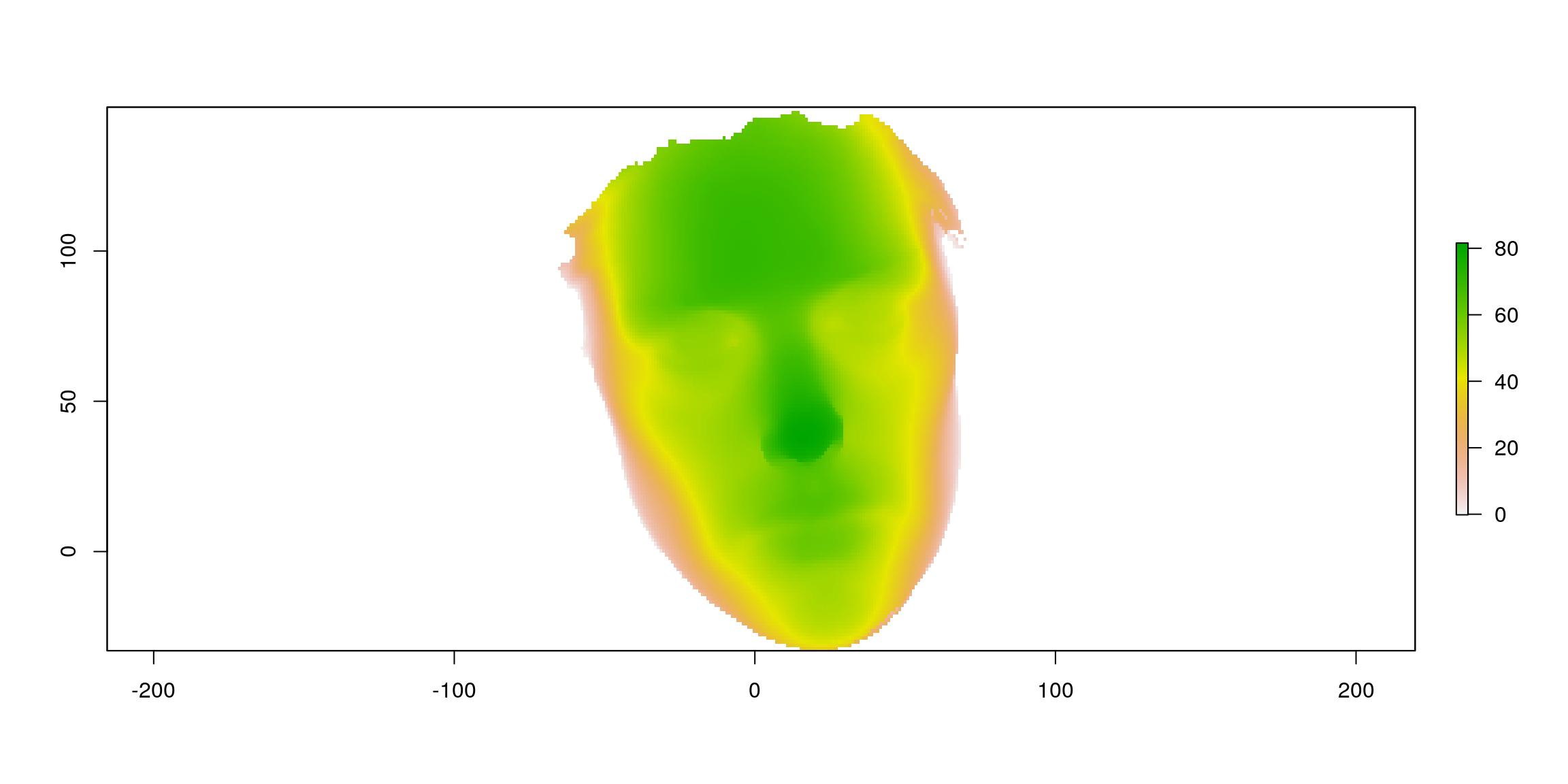
Rendre le raster avec {rayshader}
Il est facile de transformer un raster en une matrice utilisable par {rayshader}. Il suffit de transposer un as.matrix().
datamat <- t(as.matrix(hum_mesh_r))
# Rayshade raster
zscale <- 0.1
ambmat <- ambient_shade(datamat, zscale = zscale)
raymat <- ray_shade(datamat, zscale = zscale, lambert = TRUE,
                    sunangle = 45)

ray_image <- datamat %>%
  sphere_shade(texture = "unicorn") %>%
  add_shadow(raymat, max_darken = 0.1) %>%
  add_shadow(ambmat, max_darken = 0.5)

plot_map(ray_image)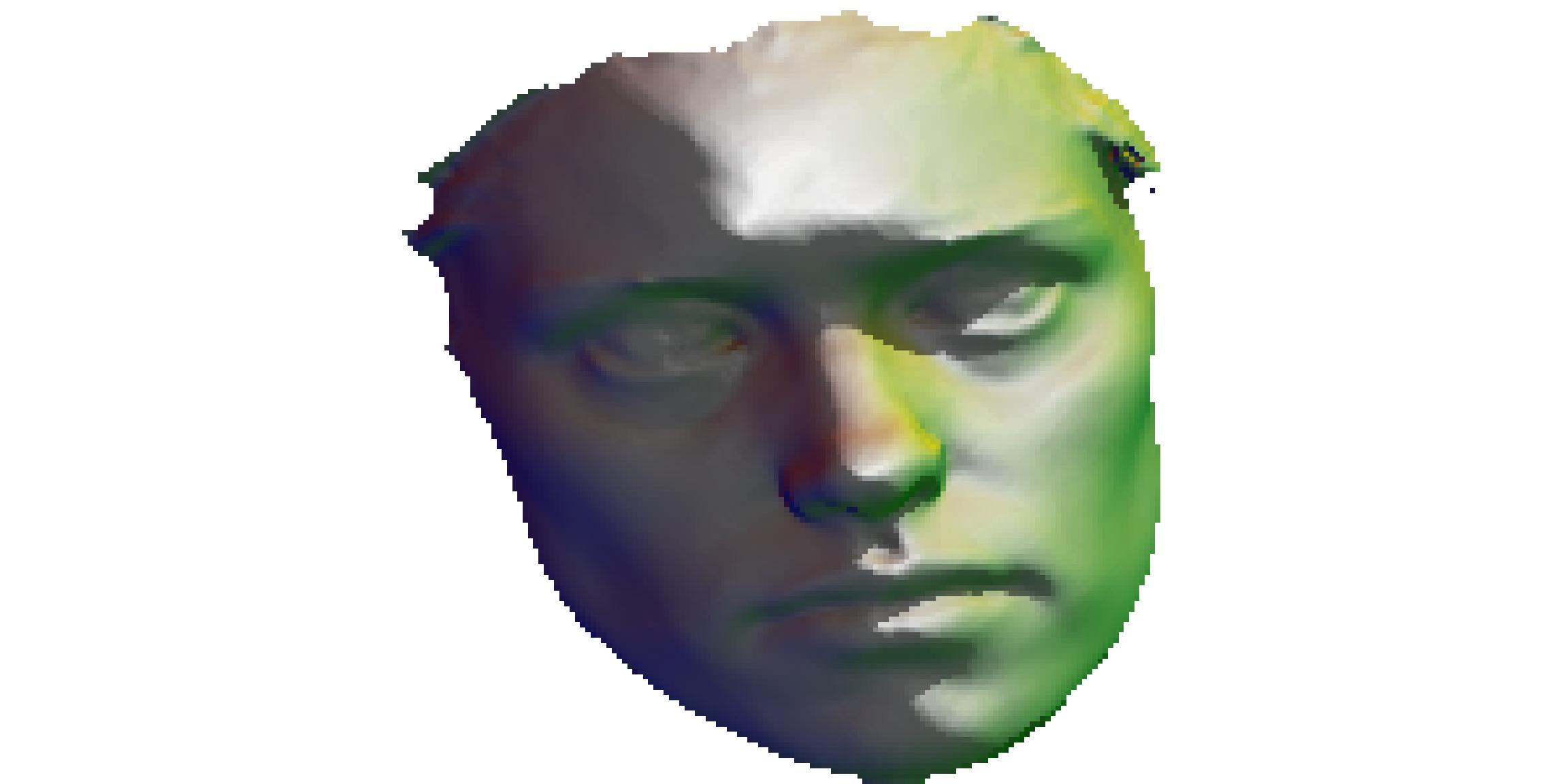
Si vous souhaitez recouvrir votre raster avec une image qui n’a rien à voir, ça demande quelques astuces. Dans le package {mesh2ray}, vous pourrez utiliser la fonction stack_to_ray() pour ré-échantillonner votre image aux dimensions du raster et récupérer la matrice de couleurs nécessaires à {rayshader}.
Par ailleurs, une sortie {rayshader} ne serait pas digne de ce nom sans un gif…
r_img <- stack(file.path(extraWD, "ThinkR_logo_500px.png"))
hum_mesh_img <- stack_to_ray(hum_mesh_r, r_img)

# Rayshade raster
zscale <- 0.25
ambmat <- ambient_shade(hum_mesh_img$elevation, zscale = zscale)
raymat <- ray_shade(hum_mesh_img$elevation, zscale = zscale, lambert = TRUE)

ray_image_overlay <- hum_mesh_img$elevation %>%
  sphere_shade(texture = "imhof4") %>%
  add_overlay(hum_mesh_img$overlay, alphalayer = 0.99) %>% # Note overlay
  add_shadow(raymat, max_darken = 0.01) %>%
  add_shadow(ambmat, max_darken = 0.5) # %>%
# add_water(watermap, color = "#57B6FF")

# transform as gif
path_gif <- file.path(extraWD, "face.gif")
if (!file.exists(path_gif)) {
  # Add some movement
  th <- seq(-50, 50, length.out = 20)
  ph <- seq(80, 90, length.out = 20)
  move <- data.frame(theta = c(th, rev(th)), phi = c(ph, rev(ph)))

  n_frames <- nrow(move)
  dir.create(file.path(extraWD, "face_gif"), showWarnings = FALSE)
  img_frames <- file.path(
    extraWD, "face_gif",
    paste0("face", formatC(seq_len(n_frames), width = 3, flag = "0"), ".png"))

  # create all frames
  for (i in seq_len(n_frames)) {
    ray_image_overlay %>%
      plot_3d(hum_mesh_img$elevation, zscale = zscale, windowsize = c(1000, 1000),
              soliddepth = -max(hum_mesh_img$elevation, na.rm = TRUE)/zscale,
              theta = move$theta[i], phi = move$phi[i], zoom = 0.30, fov = 20
      )

    rgl::snapshot3d(img_frames[i])
    rgl::clear3d()
  }
  rgl::rgl.close()

  magick::image_write_gif(magick::image_read(img_frames),
                          path = path_gif,
                          delay = 6/n_frames)
}
file.copy(file.path(extraWD, "face.gif"),
          file.path(glue("../../static{StaticImgWD}/face.gif")),
          overwrite = TRUE)
Rendre un mesh3d avec {rayrender}
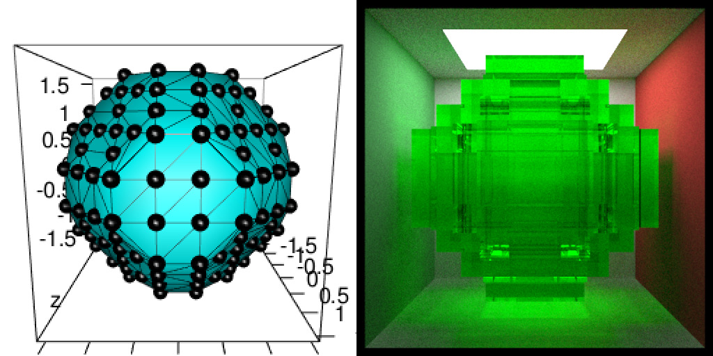
{rayrender} peut dessiner des cubes en connaissant la position du centre du cube et ses dimensions en x, y et z. Pour un rendu avec un mesh triangulaire, je l’ai imaginé comme une image voxelisées. C’est-à-dire une image pixelisée mais en 3D, un peu comme on l’a fait pour la transformation en raster 2D. {Rvcg} a des outils puissants pour travailler avec de très gros mesh.
can draw cubes using position of its center and dimensions in x, y and z. To render a triangluar mesh, I imagined it as a voxelized image. It is the same as in 2D dimension when I transformed the mesh into a 2D regular grid, except this will be a 3D regular grid.
{Rvcg} has powerful tools to work with big mesh. Par exemple, la fonction vcgUniformRemesh() rééchantillonne un mesh de manière régulière. Cela signifie que les nouveaux points d’un mesh régulier peuvent être utilisés comme le centres de mes cubes. Il suffit ensuite de calculer la distance entre chaque centre en x, y et z pour construire les cubes.
Étapes de la méthode de mesh3d vers {rayrender}
Les images ci-dessous montrent la procédure complète sur un petit mesh avec une faible résolution :
- Rééchantillonnage régulier du mesh 3d avec
Rvcg::vcgUniformRemesh. - Extraction des informations du mesh régulier avec
mesh2ray::mesh_to_cubes(qui inclutvcgUniformRemesh) - Ajout des cubes à la scène avec
mesh2ray::add_cubes_to_scene. - Tracez la scène en utilisant {rayrender}
# Create simple mesh
simple_mesh <- Rvcg::vcgIcosahedron()

# _plot3d
plot3d(simple_mesh, col = "cyan")
aspect3d("iso")
plot3d(simple_mesh, type = "wire", add = TRUE)
plot3d(t(simple_mesh$vb), type = "s", radius = 0.1, add = TRUE)
view3d(theta = 0, phi = 10, zoom = 0.6, fov = 80)
# _snapshot
rgl.snapshot(filename = file.path(extraWD, "rayrender-simple-1-mesh.png"))
rgl::rgl.close()

# 1. Uniformely resample mesh
# _vcgUniformRemesh is included in mesh_to_cubes()
simple_resample <- vcgUniformRemesh(simple_mesh, voxelSize = 0.5, multiSample = TRUE,
                                discretize = TRUE)

plot3d(simple_resample, col = "cyan")
aspect3d("iso")
plot3d(simple_resample, type = "wire", add = TRUE)
plot3d(t(simple_resample$vb), type = "s", radius = 0.1, add = TRUE)
view3d(theta = 0, phi = 10, zoom = 0.6, fov = 80)
# _snapshot
rgl.snapshot(filename = file.path(extraWD, "rayrender-simple-2-regularmesh.png"))
rgl::rgl.close()

# 2. Calculate cube positions in a specific scene
# _vcgUniformRemesh is included in mesh_to_cubes()
simple_cubes <- mesh2ray::mesh_to_cubes(simple_mesh, voxelSize = 0.5, scene_dim = c(80, 475))

# 3. Draw with rayrender
# _scene
scene <- generate_cornell(lightintensity = 10)
# _add cubes on scene
scene <- mesh2ray::add_cubes_to_scene(scene, cubes = simple_cubes,
                                      material = dielectric(color = "green"))
# _draw scene /!\ long calculation /!\
if (!file.exists(file.path(extraWD, "rayrender-simple-3-scene.png"))) {
  options(cores = 4)
  render_scene(scene, lookfrom = c(278, 278, -800) ,
               lookat = c(278, 278, 0), fov = 40, ambient_light = FALSE,
               samples = 500, parallel = TRUE, clamp_value = 5,
               filename =  file.path(extraWD, "rayrender-simple-3-scene.png"))
}

# Image montage
img_frames <- list.files(extraWD, pattern = "rayrender-simple", full.names = TRUE)
image_append(image_scale(image_read(img_frames), "400"))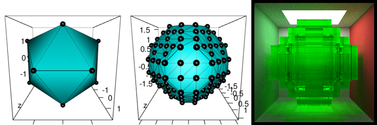
Figure 2: Low resolution rayrendering. a. mesh3d, b. regularly sampled mesh, c. rayrendered regularly sampled mesh
Appliquer la voxélisation sur le visage humain et définir les couleurs
Les étapes sont les mêmes que dans le petit exemple ci-dessus. Nous utilisons une résolution plus élevée pour obtenir une forme finale beaucoup plus proche de l’original.
Cependant, je voulais ajouter des couleurs à certains cubes et pour ça, j’ai fait quelques dessins manuels sur des tracés 2D. Après quelques manipulations de données géographiques et de polygones avec {sf}, je peux obtenir une version colorée du visage en 2D.
# voxelisation
data(humface)
human_cubes <- mesh2ray::mesh_to_cubes(humface, voxelSize = 0.5, scene_dim = c(20, 535))

# Define colours areas manually
polygon_contours_file <- file.path(extraWD, "polygon_contours.rds")
if (!file.exists(polygon_contours_file)) {
  # Manually draw polygons
  plot(human_cubes$cube_center$x, human_cubes$cube_center$y, pch = 20, cex = 0.5)

  eye1 <- raster::drawPoly(col = "blue")
  eye2 <- raster::drawPoly(col = "blue")
  mouth <- raster::drawPoly(col = "red")
  front <- raster::drawPoly(col = "green")

  polygon_contours <- list(eye1 = eye1, eye2 = eye2, mouth = mouth, front = front)
  # Transform as sf polygon
  polygon_contours_sf <- polygon_contours %>%
  purrr::map2(names(polygon_contours),
              ~sf::st_as_sf(.x) %>% mutate(name = .y)) %>%
  do.call("rbind", .)

  readr::write_rds(polygon_contours_sf, polygon_contours_file)
} else {
  polygon_contours_sf <- readr::read_rds(polygon_contours_file)
}

# Transform cubes as sf for intersection with contours
human_colours <- human_cubes$cube_center %>%
  sf::st_as_sf(coords = c("x", "y"), remove = FALSE) %>%
  sf::st_join(polygon_contours_sf) %>%
  mutate(colours = case_when(
    name %in% c("eye1", "eye2") ~ "blue",
    name == "mouth" ~ "red",
    name == "front" ~ "ivory",
    TRUE ~ "grey"
  )) %>%
  as_tibble()

# Explore the 3D points and color
plot3d(t(human_cubes$mesh_resample$vb), type = "s", radius = 1,
       col = human_colours$colours)
aspect3d("iso")
view3d(theta = 0, phi = 10, zoom = 0.6, fov = 80)
# _snapshot
rgl.snapshot(filename = file.path(tmpImgWD, "figure-html/humcolours.png"))
rgl::rgl.close()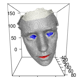
Definir le matériel de chaque cube
Je peux créer un tibble contenant le type de matériel de chaque cube à dessiner.
# All types of cubes
colours_cubes <- bind_rows(
  lambertian(color = "ivory"),
  dielectric(color = "#2E7BE6"),
  dielectric(color = "#2E7BE6"),
  dielectric(color = "#DB3B3B"),
  dielectric()
) %>%
  mutate(name = c(NA, "eye1", "eye2", "mouth", "front"))

# Join with table of colours
human_materials <- dplyr::select(human_colours, name) %>%
  left_join(colours_cubes, by = "name") %>%
dplyr::select(-name)human_materials## # A tibble: 245,975 x 12
## type properties checkercolor noise noisephase noiseintensity noisecolor
## <chr> <list> <list> <dbl> <dbl> <dbl> <list>
## 1 lamb… <dbl [3]> <dbl [2]> 0 0 10 <dbl [3]>
## 2 lamb… <dbl [3]> <dbl [2]> 0 0 10 <dbl [3]>
## 3 lamb… <dbl [3]> <dbl [2]> 0 0 10 <dbl [3]>
## 4 lamb… <dbl [3]> <dbl [2]> 0 0 10 <dbl [3]>
## 5 lamb… <dbl [3]> <dbl [2]> 0 0 10 <dbl [3]>
## 6 lamb… <dbl [3]> <dbl [2]> 0 0 10 <dbl [3]>
## 7 lamb… <dbl [3]> <dbl [2]> 0 0 10 <dbl [3]>
## 8 lamb… <dbl [3]> <dbl [2]> 0 0 10 <dbl [3]>
## 9 lamb… <dbl [3]> <dbl [2]> 0 0 10 <dbl [3]>
## 10 lamb… <dbl [3]> <dbl [2]> 0 0 10 <dbl [3]>
## # … with 245,965 more rows, and 5 more variables: image <list>,
## # lightintensity <lgl>, fog <lgl>, fogdensity <dbl>, implicit_sample <lgl>Dessiner la scène complète
L’objet voxélisé human_cubes doit être ajouté à une scène vierge à l’aide de mesh2ray::add_cubes_to_scene en utilisant le tibble de matériels créé. Dessiner la scène nécessite un peu de temps. Soyez patients… Vous pouvez paralléliser le calcul pour accélérer un peu les choses.
# 3. Draw with rayrender
if (!file.exists(file.path(extraWD, "rayrender-human-scene.png"))) {
  # _scene
  scene <- generate_cornell(lightintensity = 20)
  # _add cubes on scene with material data.frame /!\ A little long /!\
  scene <- mesh2ray::add_cubes_to_scene(scene, cubes = human_cubes,
                                        material = human_materials)

  # _draw scene /!\ long calculation /!\
  options(cores = 4)
  render_scene(scene, width = 600, height = 600,
               lookfrom = c(278, 278, -800) ,
               lookat = c(278, 278, 0), fov = 40, ambient_light = FALSE,
               samples = 500, parallel = TRUE, clamp_value = 5,
               filename =  file.path(tmpImgWD, "figure-html/rayrender-human-scene.png"))
}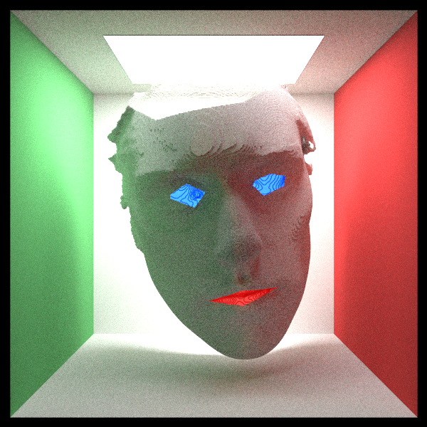
Tada ! Maintenant, c’est à vous ! Bien que ces deux packages {rayshader} et {rayrender} soit jeunes, ils ouvrent déjà beaucoup de possibilités. Je suis sûr qu’il y aura de grandes innovations autour. Et rappelez vous toujours de prendre du temps pour prendre du plaisir ! R est aussi fait pour ça !
Ressources
Packages mis en avant ici :
- {rayshader} and {rayrender} for ray tracing. Have a look at Tyler Morgan blog here.
- {Morpho} and {Rvcg} for 3d mesh manipulation. Have a look at Stefan Schlager blog here.
- {mesh2ray} that I share on github
Liste complète des packages utilisés dans cet article :
attachment::att_from_rmd("2019-04-02-mesh3d-rayshader-and-rayrender.Rmd")## [1] "raster" "dplyr" "Rvcg" "rgl" "rayshader"
## [6] "rayrender" "mesh2ray" "magick" "readr" "attachment"Comme toujours, le script R complet de cet article est sur mon dépôt Github Blog tips.
Citation :
Merci de citer ce travail avec :
Rochette Sébastien. (2019, avr.. 10). "Utiliser des objets mesh3d avec rayshader et rayrender". Retrieved from https://statnmap.com/fr/2019-04-02-mesh3d-rayshader-et-rayrender/.
Citation BibTex :
@misc{Roche2019Utili,
    author = {Rochette Sébastien},
    title = {Utiliser des objets mesh3d avec rayshader et rayrender},
    url = {https://statnmap.com/fr/2019-04-02-mesh3d-rayshader-et-rayrender/},
    year = {2019}
  }