#30DayMapChallenge: 30 days building maps (2) - tmap

Packages

library(dplyr)
library(sf)
library(raster)
library(readr)
library(tmap)
library(xml2)
library(purrr)
# remotes::install_github("tylermorganwall/rayshader")
library(rayshader)

## Customize
my_blue <- "#1e73be"
# Test for font family
# extrafont::font_import(prompt = FALSE)
font <- extrafont::choose_font(c("Nanum Pen", "Lato", "sans"))

Data: Transform France into a regular grid of hexagons

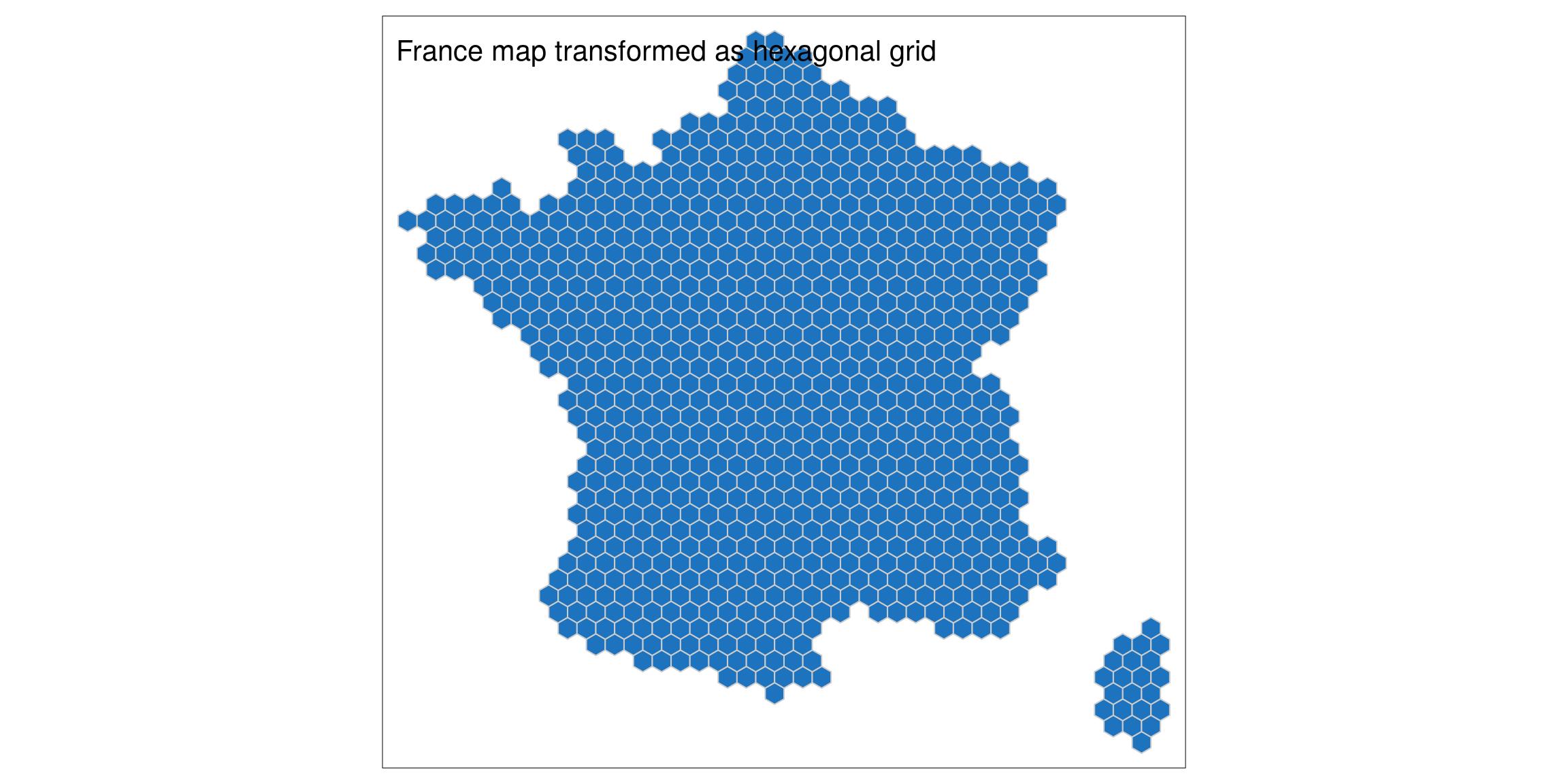
• Get World data in {tmap} package
• Get France shapefile
• Transform France into a regular grid of hexagons

# extraWD <- "." # Uncomment for the script to work
data(World)
# Read shapefile "Departement.shp"
France_L93 <- st_read(file.path(extraWD, "DEPARTEMENT.shp"), quiet = TRUE)

# Transform as hex polygon grid
#' @param x a sf object
transform_to_hex <- function(x) {
x %>% 
  st_make_grid(what = "polygons", square = FALSE,
               n = c(40, 20)) %>% 
  st_sf() %>% 
  mutate(id_hex = 1:n()) %>% 
  dplyr::select(id_hex, geometry)
}
France_hex <- transform_to_hex(France_L93)

tm_shape(France_hex) +
  tm_fill(col = my_blue) +
  tm_borders(col = "grey80") +
  tm_legend(
    title = "France map transformed as hexagonal grid"
  )

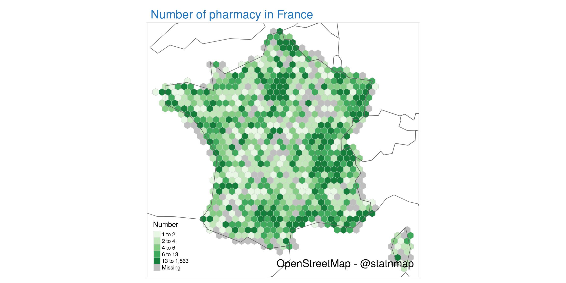
Green: Plot a regular grid of hexagons in {tmap}

Now that I have access to OpenDataSoft datasets, I will cheat a little on the Challenge and use it for my following maps. What could be green? Pharmacy is a good candidate.

As I will use again the code to transform OSM data as shapefiles for the next challenge, I can transform it as a function.

#' @param amenity Character. An amenity.
#' @param file_amenity path to where to save downloaded data
#' @param hex Hexagonal polygon grid
get_and_sf <- function(amenity, file_amenity, hex) {
  if (!file.exists(file_amenity)) {
    # devtools::install_github("tutuchan/fodr")
    # portal <- fodr::fodr_portal("ods")
    poi <- fodr::fodr_dataset("ods", "points-dinterets-openstreetmap-en-france")
    
    # Get amenity
    amenity <- poi$get_records(refine = list(amenity = amenity))
    
    amenity_chr <- amenity %>% 
      dplyr::select(-geo_shape, -other_tags)
    
    write_csv(amenity_chr, file_amenity)
    
  } else {
    amenity_chr <- read_csv(file_amenity)
  }
  
  amenity_sf_l93 <- amenity_chr %>% 
    st_as_sf(coords = c("lng", "lat"), crs = 4326) %>% 
    st_transform(crs = 2154)
  
  # Join amenity wth hex and count
  amenity_hex_l93 <- st_join(amenity_sf_l93, hex)
  amenity_hex_count <- amenity_hex_l93 %>% 
    st_drop_geometry() %>% 
    count(id_hex)
  
  # Join hex with bars count
  France_hex_amenity <- hex %>% 
    left_join(amenity_hex_count)
}

This is a new week, so let’s add a supplementary challenge. This week I create maps with {tmap} instead of {ggplot2}.

France_hex_pharmacy <- get_and_sf(
  amenity = "pharmacy",
  file_amenity = file.path(extraWD, "pharmacy.csv"),
  hex = France_hex)

tm_shape(France_hex_pharmacy, is.master = TRUE) +
  tm_fill(col = "n", palette = "Greens",
          style = "quantile",
          title = "Number") +
  tm_borders(col = "grey80", lwd = 0.5) +
tm_shape(World) +
  tm_borders() +
  tm_credits("OpenStreetMap - @statnmap",
             position = c("RIGHT", "BOTTOM"),
             size = 2) +
  tm_legend(
    main.title = "Number of pharmacy in France",
    main.title.color = my_blue
    # main.title.size = 1
  )

Yellow: Plot a grid of points on hexagonal grid

The previous map is not the most wonderful map I ever realised… I will use this week to go a little further in the use of {tmap}. I continue to use OpenDataSoft data, this time with post office data, as this is the yellow challenge.

• Colour shades is not the best way to visualize differences. I will use centroids of hexagons to create a point map.
• In the previous map, I could not fill the polygons of other European countries. This was because the layer used as master is the map of France and it does not have the same projection as the one of the World. The on-the-fly projection of the world map by {tmap} didn’t really work. In cartography, it is very often a problem with projections! Go back to Introduction to mapping with {sf} & Co. to learn more. To avoid this problem, I filtered only European countries from the “World” dataset and projected them onto France’s projection system. As we are going to zoom in close to France, I allow myself to do so…

France_hex_post <- get_and_sf(
  amenity = "post_office",
  file_amenity = file.path(extraWD, "post_office.csv"),
  hex = France_hex)

# Transform as points
France_hexcenter_post <- France_hex_post %>% 
  st_centroid()
lim.n <- range(France_hexcenter_post$n, na.rm = TRUE)


# Transform to projection of the master map for correct colour fill
Europe <- World %>% 
  filter(continent == "Europe") %>% 
  st_transform(crs = st_crs(France_hex_post))

# tmap
tm <- tm_shape(Europe) +
  tm_fill(col = "#38424f") +
  tm_borders(col = "grey80") +
tm_shape(France_hexcenter_post, is.master = TRUE) +
  tm_bubbles(size = "n", col = "#ffff33", alpha = 0.75,
             border.col = NA, shape = 20, scale = 3,
             title.size = "Number", 
             legend.size.is.portrait = TRUE) +
  tm_credits("OpenStreetMap - {tmap} - @statnmap",
             position = c(0.38, -0.01),
             size = 1.3, fontfamily = "Nanum Pen",
             col = "grey90") +
  tm_layout(
    main.title = "Number of recorded post offices in France",
    main.title.color = my_blue,
    main.title.fontfamily = "Nanum Pen",
    main.title.size = 1.75,
    # Margin to allow legend
    inner.margins = c(0, 0.2, 0, 0),
    # Colours
    outer.bg.color = c("#E6EFFA"),
    bg.color = "grey60",
    legend.title.fontfamily = "Nanum Pen",
    legend.title.size = 1.5,
    legend.bg.color = "grey80",
    legend.bg.alpha = 0.5
  )

tmap_save(tm, filename = file.path(extraWD, "yellow.jpg"),
          width = 1024, height = 512, units = "px",
          dpi = 100)

tm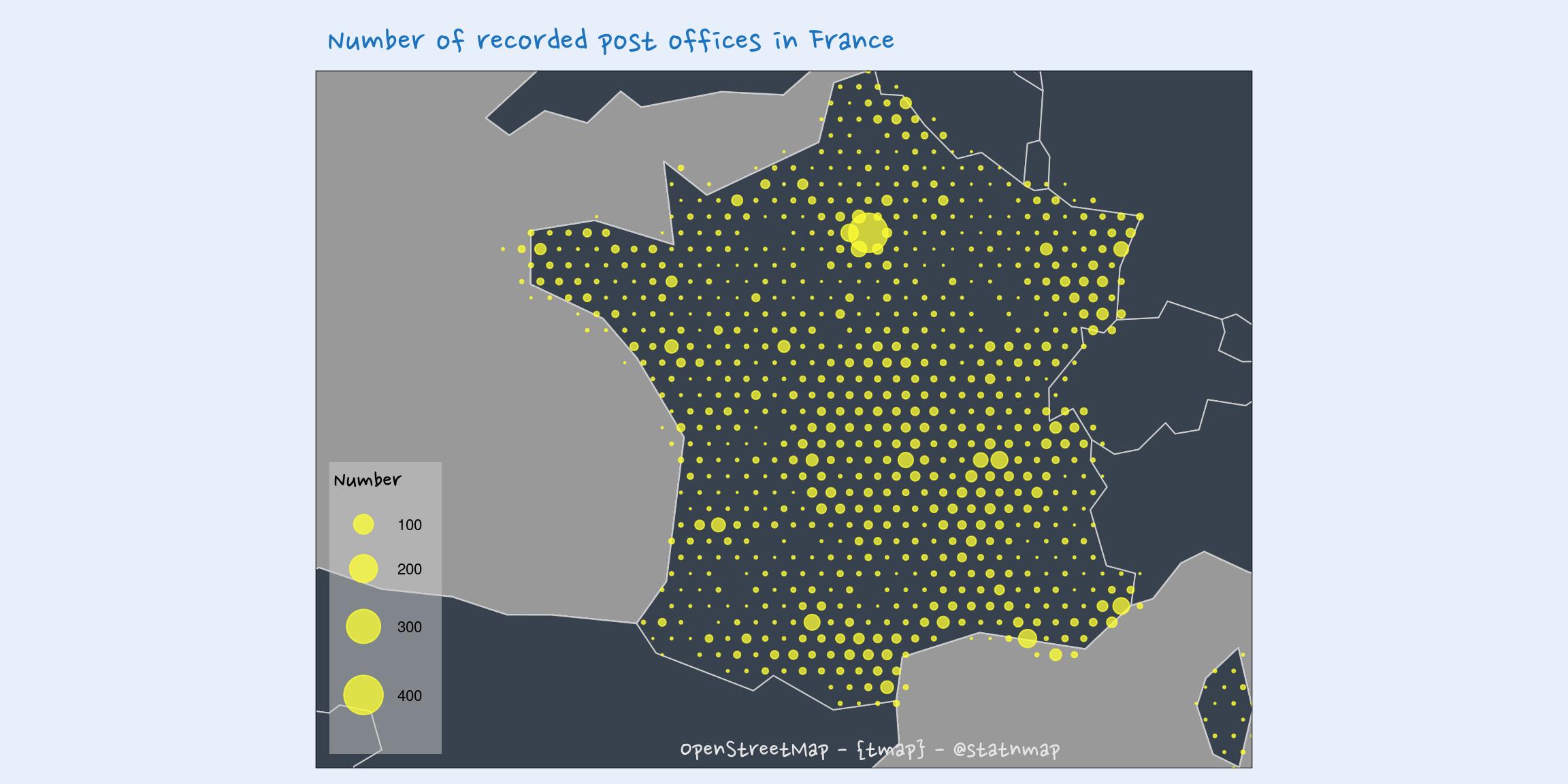

Black and White: Add user-specific icons to a map with {tmap}

Let’s map the distribution of French Tax offices. Data is available from Service-public.fr - Annuaire de l’administration - Base de données locales. This datasets are stored as XML files in different directories for each department, and different files for each office.

• Extraction of coordinates from XML files, using {xml2}
• Extraction of all offices of all department
• Use of a more precise world map from {rnaturalearth} to replace Europe map used previously

# Get data if not already dowloaded ----
data_untared <- file.path(extraWD, "all_20191107")
if (!dir.exists(data_untared)) {
  databz2 <- file.path(extraWD, "all_latest.tar.bz2")
  download.file(
    "http://lecomarquage.service-public.fr/donnees_locales_v2/all_latest.tar.bz2", destfile = databz2)
  utils::untar(databz2, exdir = extraWD)
}

# Get data from xml ----
#' Get infos from one xml
#' @param xml_path Path to one xml
#' @return a tibble
get_infos <- function(xml_path) {
  # which_tresor <- 1
  # xml_path <- tresor[which_tresor]
  xml_content <- read_xml(xml_path)
  lat <- xml_content %>% 
    xml_find_first(xpath = ".//Latitude") %>% 
    xml_double() 
  long <- xml_content %>% 
    xml_find_first(xpath = ".//Longitude") %>% 
    xml_double()
  codepostal <- xml_content %>% 
    xml_find_first(xpath = ".//CodePostal") %>% 
    xml_text()
  nomcommune <- xml_content %>% 
    xml_find_first(xpath = ".//NomCommune") %>% 
    xml_text()
  
  tibble(
    x = long,
    y = lat, 
    code_postal = codepostal,
    nom_commune = nomcommune,
    file = basename(xml_path)
  )
}

# Get all data from all interesting xml
directory <- file.path(data_untared, "organismes")
all_dpt <- list.dirs(directory, full.names = TRUE, recursive = FALSE)

all_positions <- map_dfr(all_dpt, function(one_dpt) {
  interest <- list.files(one_dpt,
                         pattern = "^tresorerie.*\\.xml$",
                         full.names = TRUE)
  if (length(interest) != 0) {
    map_dfr(interest, get_infos)
  } else {NULL}
})

# Transform as spatial data
all_positions_sf <- all_positions %>% 
  filter(!is.na(x) & !is.na(y)) %>% 
  st_as_sf(coords = c("x", "y"), crs = 4326)

# Transform to projection of the master map for correct colour fill
world_ne <- rnaturalearth::ne_countries(scale = 10 , returnclass = "sf")

tm1 <- tm_shape(world_ne, projection = "wintri") +
  tm_fill() +
tm_shape(all_positions_sf) +
  tm_symbols(
    shape = leaflet::icons(
      file.path(extraWD, "Logo_Tresor_public_50x50.png")),
    size = 0.1
    )
tm1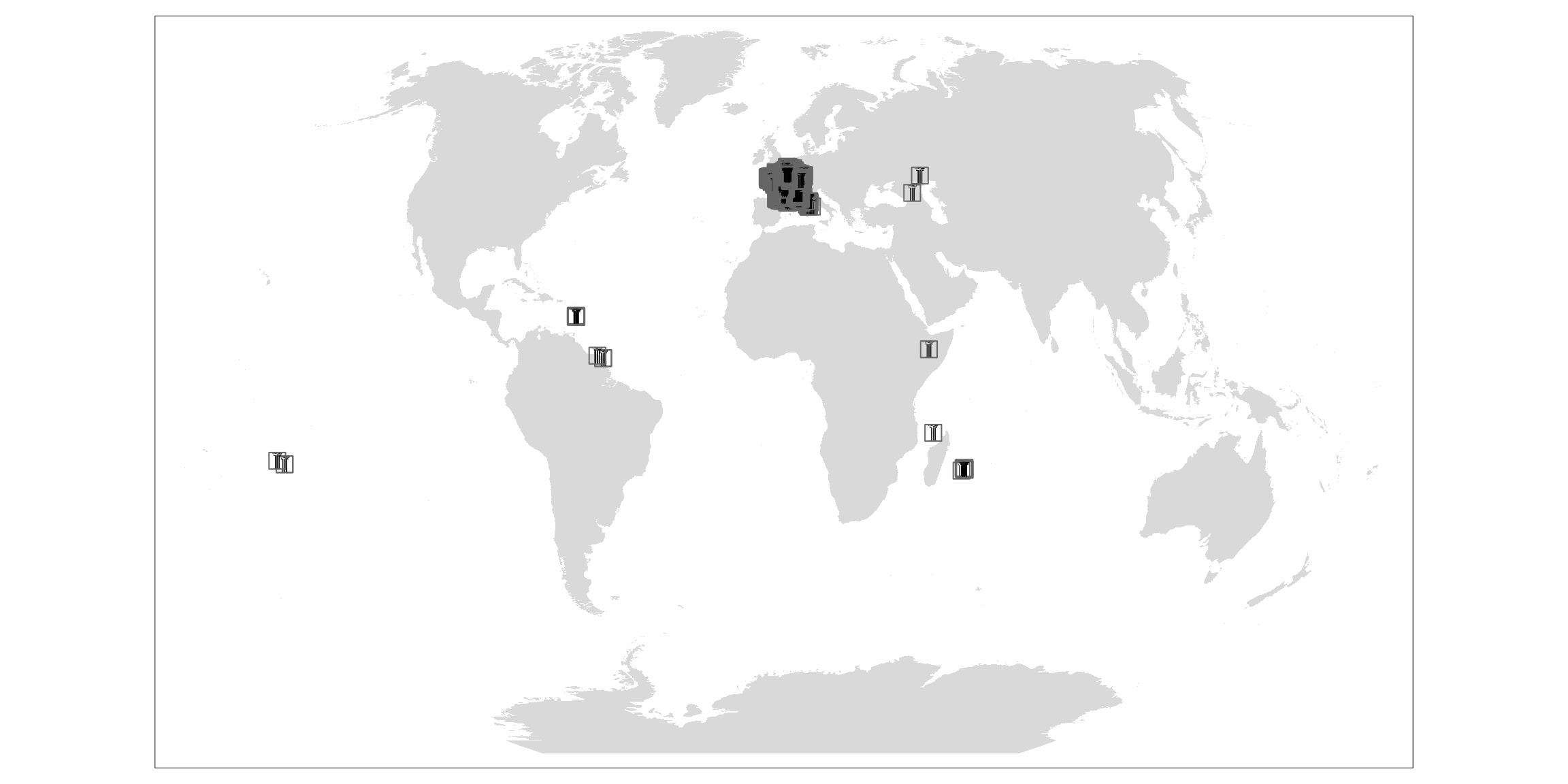

# Metropolitan France only
all_france_metro <- all_positions_sf %>% 
  st_transform(st_crs(France_L93)) %>% 
  st_crop(France_L93)

europe_ne <- world_ne %>% 
  filter(continent == "Europe")

# Point with the big logo
logo <- st_point(c(100000, 6500000)) %>% 
  st_sfc(crs = st_crs(France_L93))

# Map
tm2 <- tm_shape(europe_ne) +
  tm_borders(col = "grey90") +
tm_shape(France_L93, is.master = TRUE) +
  tm_fill(col = "white") +
tm_shape(logo) +
  tm_symbols(
    shape = tmap_icons(
    file.path(extraWD, "Logo_Tresor_public_50x50.png")),
    size = 3) +
tm_shape(all_france_metro) +
  tm_symbols(
    shape = tmap_icons(
      file.path(extraWD, "Logo_Tresor_public_50x50.png")),
    size = 0.05,
    border.col = NA, border.lwd = 0,
    alpha = 1
  ) +
  tmap_icons(
      file.path(extraWD, "Logo_Tresor_public_50x50.png"),
      iconAnchorX = -4, iconAnchorY = 50) +
  tm_credits("service-public.fr - {tmap} - @statnmap",
             position = c(0.38, -0.01),
             size = 1.3, fontfamily = "Nanum Pen",
             col = "grey90") +
  tm_layout(
    main.title = "Tax offices in France",
    main.title.color = my_blue,
    main.title.fontfamily = "Nanum Pen",
    main.title.size = 1.75,
    # Margin to allow legend
    inner.margins = c(0, 0.2, 0, 0),
    # Colours
    outer.bg.color = c("#E6EFFA"),
    bg.color = my_blue #"grey60"
  )

tmap_save(tm2, filename = file.path(extraWD, "black_white.jpg"),
          width = 1024, height = 512, units = "px",
          dpi = 100)

tm2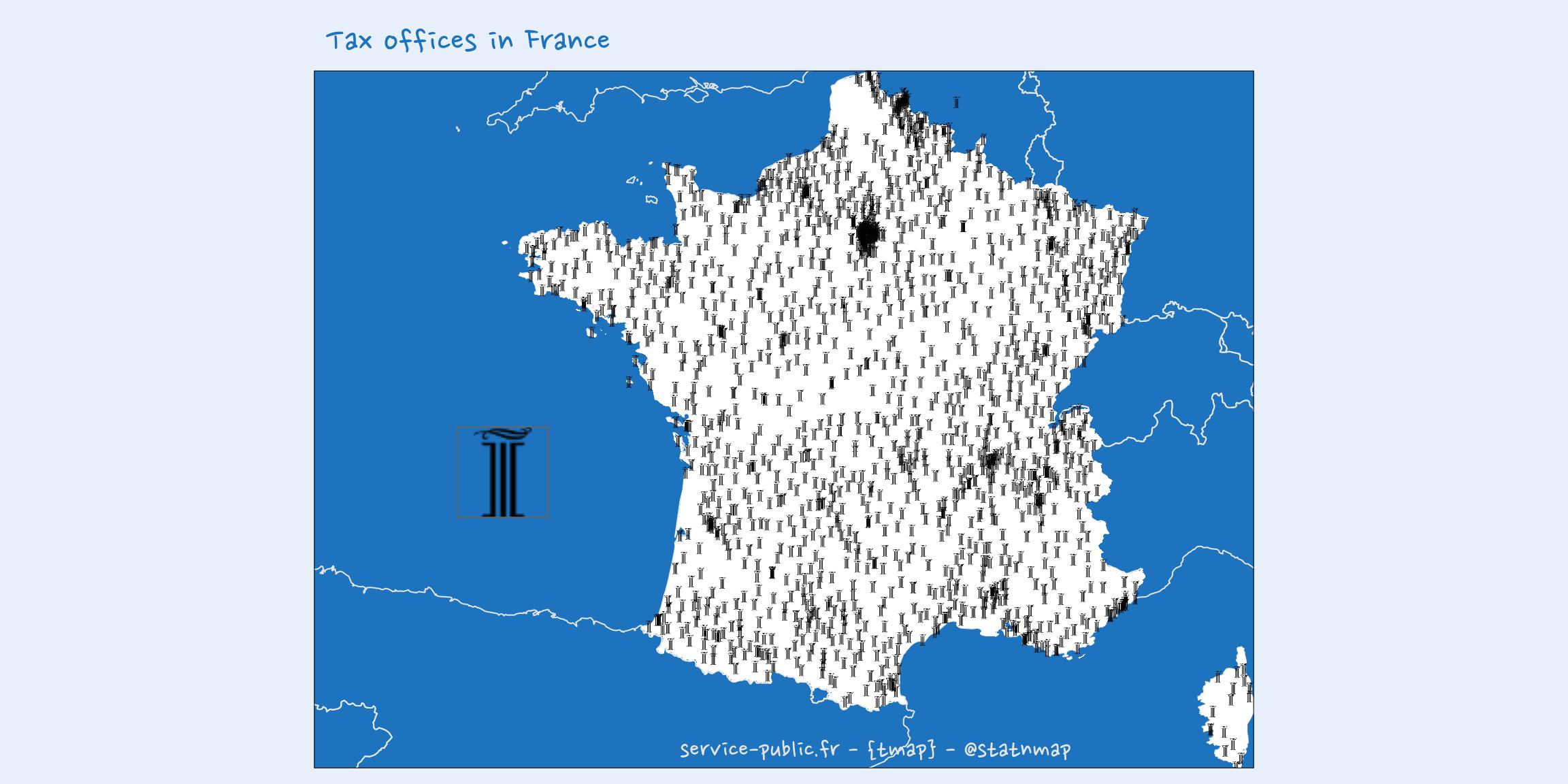

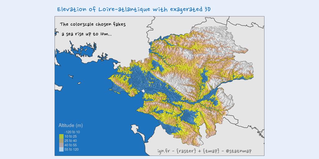
Elevation: Overlay multiple rasters on a map using {tmap}

{tmap} is also really good at plotting raster datasets. The combination of multiple raster files is also quite easy. Here, I show the elevation data for Loire-atlantique department over its hillshaded raster to give an impression of 3D observation.

• Read raster of Altitude
  • Reproject raster of Altitude. Be careful when you reproject raster datasets, you recalculate a brand new raster, with cell position that have changed compared to the original dataset.
• Calculate sun position for one point and date using {cartomisc}
  • remotes::install_github("statnmap/cartomisc")
• Calculate hillshade with {raster}
• Choose colors so that we can fake a rise of sea elevation up to 10m

# Reproject
Alti_44_wgs84 <- raster(file.path(extraWD, "Alti_44_L93.tif")) %>% 
  projectRaster(crs = "+init=epsg:4326")

# Calculate sun position in the center with {cartomisc}
Sun <- cartomisc::sun_position(year = 2019, month = 5, day = 3,
                   hour = 16, min = 30, sec = 0,
                   long = mean(bbox(Alti_44_wgs84)[1,]),
                   lat = mean(bbox(Alti_44_wgs84)[2,])
                   )
# Calculate hillShade
slope_44_wgs84 <- terrain(Alti_44_wgs84, opt = "slope")
aspect_44_wgs84 <- terrain(Alti_44_wgs84, opt = "aspect")
hillShade_44_wgs84  <- hillShade(
  slope = slope_44_wgs84 * 40, aspect = aspect_44_wgs84, 
  angle = Sun$elevation, direction = Sun$azimuth,
  overwrite = TRUE)

# Graph
tm <- tm_shape(France_L93) +
  tm_fill("grey90") +
  tm_borders(col = "grey20") +
tm_shape(hillShade_44_wgs84, is.master = TRUE) +
  tm_raster(
        style = "pretty",
        palette = "-Greys",
        legend.show = FALSE
        ) +
tm_shape(Alti_44_wgs84) +
  tm_raster(
        style = "fixed",
        palette = c(my_blue, terrain.colors(5)[2:5]),
        breaks = c(-120, 10, 25, 40, 55, 120),
        alpha = 0.70,
        title = "Altitude (m)"
        ) +  
  tm_credits("ign.fr - {raster} + {tmap} - @statnmap",
             position = c(0.48, -0.01),
             size = 1.3, fontfamily = "Nanum Pen",
             col = "grey40") +
  tm_layout(
    main.title = "Elevation of Loire-atlantique with exagerated 3D",
    main.title.color = my_blue,
    main.title.fontfamily = "Nanum Pen",
    main.title.size = 1.75,
    title = " The colorscale chosen fakes\n  a sea rise up to 10m...",
    title.fontfamily = "Nanum Pen",
    # Margin to allow legend
    inner.margins = c(0, 0.2, 0.05, 0),
    # Colours
    outer.bg.color = c("#E6EFFA"),
    bg.color = my_blue, #"grey60",
    # Legend
    legend.title.color = "grey80",
    legend.text.color = "grey80",
    legend.position = c("left","bottom")
  )

tmap_save(tm, filename = file.path(extraWD, "elevation.jpg"),
          width = 1024, height = 512, units = "px",
          dpi = 100)

tm

Movements: Transform points as lines and animate a map with {tmap}

Let’s try to follow me from 1st January to 31st December 2019. Can you guess where I live?

• Join travels and cities position
• Create lines with each “from-to” couples of points
• Duplicate points and lines to create an animation where previous lines remain on screen
• Create an animated map with {tmap} and tmap_animation(). Note that animation needs to be set with tm_facets() for each shape if required

world_ne <- rnaturalearth::ne_countries(scale = 10 , returnclass = "sf")
# Transform to projection of the master map for correct colour fill
europe_ne <- world_ne %>% 
  filter(continent == "Europe") %>% 
  st_transform(crs = 2154)

my_move <- readr::read_delim(file.path(extraWD, "movements_train_sr.txt"), delim = ";")

city_position <- readr::read_delim(file.path(extraWD, "city_positions.txt"), delim = ";")

# Transform as spatial data
my_move_sf <- my_move %>% 
  left_join(city_position, by = "city") %>% 
  st_as_sf(coords = c("lon", "lat"), crs = 4326) %>% 
  st_transform(crs = 2154)

# mapview::mapview(my_move_sf)

# Create lines with two points
# _Start
my_move_sf_head <- my_move_sf %>% 
  head(-1) %>% 
  mutate(id = 1:n())
# _End
my_move_sf_tail <- my_move_sf %>% 
  tail(-1) %>% 
  mutate(id = 1:n())

# Combine head and tail points into lines
my_move_sf_lines <- my_move_sf_head %>% 
  st_union(my_move_sf_tail, by_feature = TRUE) %>% 
  filter(id == id.1) %>% 
  st_cast("LINESTRING") 

# Duplicate lines for animation
max.frames <- nrow(my_move_sf) - 1

my_move_sf_lines_dup <- my_move_sf_lines %>% 
  mutate(
    frames = map2(id, max.frames, ~(.x:.y))
  ) %>% 
  tidyr::unnest(frames) %>% 
  dplyr::select(id, frames, everything())

# Cities duplicated for animation
my_move_sf_dup <- my_move_sf %>% 
  mutate(
    id = c(1, 1:(n()-1)), #same id for first two
    frames = map2(id, max.frames, ~(.x:.y))
  ) %>% 
  tidyr::unnest(frames) %>% 
  dplyr::select(id, frames, everything())
  
# Plot
tm <- tm_shape(europe_ne) +
  tm_fill() +
  tm_borders(col = "grey10") +
tm_shape(my_move_sf_dup, is.master = TRUE) +
  tm_dots(alpha = 0.25, size = 2) +
  # facets for animation for this shpae
  tm_facets(along = "frames", free.coords = FALSE,
            free.scales = FALSE) +
tm_shape(my_move_sf_lines_dup) +
  tm_lines(#lwd = "size",
           alpha = 0.75,
           scale = 4,
           col = "id", 
           palette = "-viridis",
           title.col = "Trip number") +
  # facets for animation for this shpae
  tm_facets(along = "frames", free.coords = FALSE,
            free.scales = FALSE) +
tm_credits("ign.fr - {raster} + {tmap} - @statnmap",
           position = c(0.48, -0.01),
           size = 1.3, fontfamily = "Nanum Pen",
           col = "grey40") +
tm_layout(
    main.title = paste("My", nrow(my_move_sf), "movements in 2019"),
    main.title.color = my_blue,
    main.title.fontfamily = "Nanum Pen",
    main.title.size = 1.75,
    title.fontfamily = "Nanum Pen",
    # Margin to allow legend
    inner.margins = c(0.15, 0.15, 0.15, 0.15),
    # Colours
    outer.bg.color = c("#E6EFFA"),
    bg.color = my_blue, #"grey60",
    # Legend
    legend.title.color = "grey80",
    legend.text.color = "grey80",
    legend.position = c("left", "center")
  )

# Animation
tmap_animation(tm, 
               filename = file.path(extraWD, "movements.gif"),
               width = 512, height = 512,# units = "px",
          dpi = 100, delay = 40)

system(paste('mogrify -fuzz 10% -layers Optimize', file.path(extraWD, "movements.gif")))
# 
# tmap_save(tm, filename = file.path(extraWD, "movements.jpg"),
#           width = 512, height = 512, units = "px",
#           dpi = 100)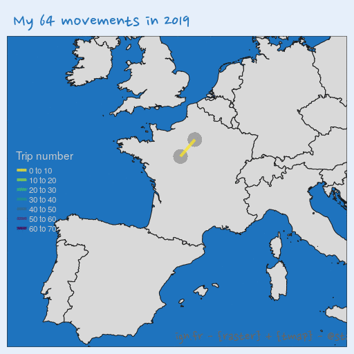

Tracks: Change spatial line width using {tmap}

Another way to explore my movements is to highlight most used railway tracks.

• Create a unique ID for each path, whatever the direction of the trip
• Count number of time each path was used
• Create a map with spatial lines with a width depending on the track use
• Add points with a color according to number of stops

# count tracks
my_tracks_count <- my_move_sf_lines %>% 
  mutate(
    unique_id = map2_chr(
      city, city.1, 
      ~paste(range(.x, .y), collapse = "-"))
  ) %>% 
  count(unique_id, sort = TRUE)

# count cities
my_cities_count <- my_move_sf %>% 
  count(city, sort = TRUE)

# Plot
tm <- tm_shape(europe_ne) +
  tm_fill() +
  tm_borders(col = "grey10") +
tm_shape(my_cities_count, is.master = TRUE) +
  tm_symbols(col = "n", size = 2,
          style = "pretty", n = 5,
          title.col = "Stop count") +
tm_shape(my_tracks_count) +
  tm_lines(lwd = "n",
           scale = 8,
           title.lwd = "Trip Count") +
tm_credits("ign.fr - {raster} + {tmap} - @statnmap",
           position = c(0.48, -0.01),
           size = 1.3, fontfamily = "Nanum Pen",
           col = "grey40") +
tm_layout(
    main.title = paste("The", nrow(my_tracks_count), "different tracks I used in 2019"),
    main.title.color = my_blue,
    main.title.fontfamily = "Nanum Pen",
    main.title.size = 1.75,
    title.fontfamily = "Nanum Pen",
    # Margin to allow legend
    inner.margins = c(0.15, 0.15, 0.15, 0.15),
    # Colours
    outer.bg.color = c("#E6EFFA"),
    bg.color = my_blue, #"grey60",
    # Legend
    legend.title.color = "grey80",
    legend.text.color = "grey80",
    legend.position = c("left", "top")
  )

tmap_save(tm, filename = file.path(extraWD, "tracks.jpg"),
          width = 1024, height = 512, units = "px",
          dpi = 100)

tm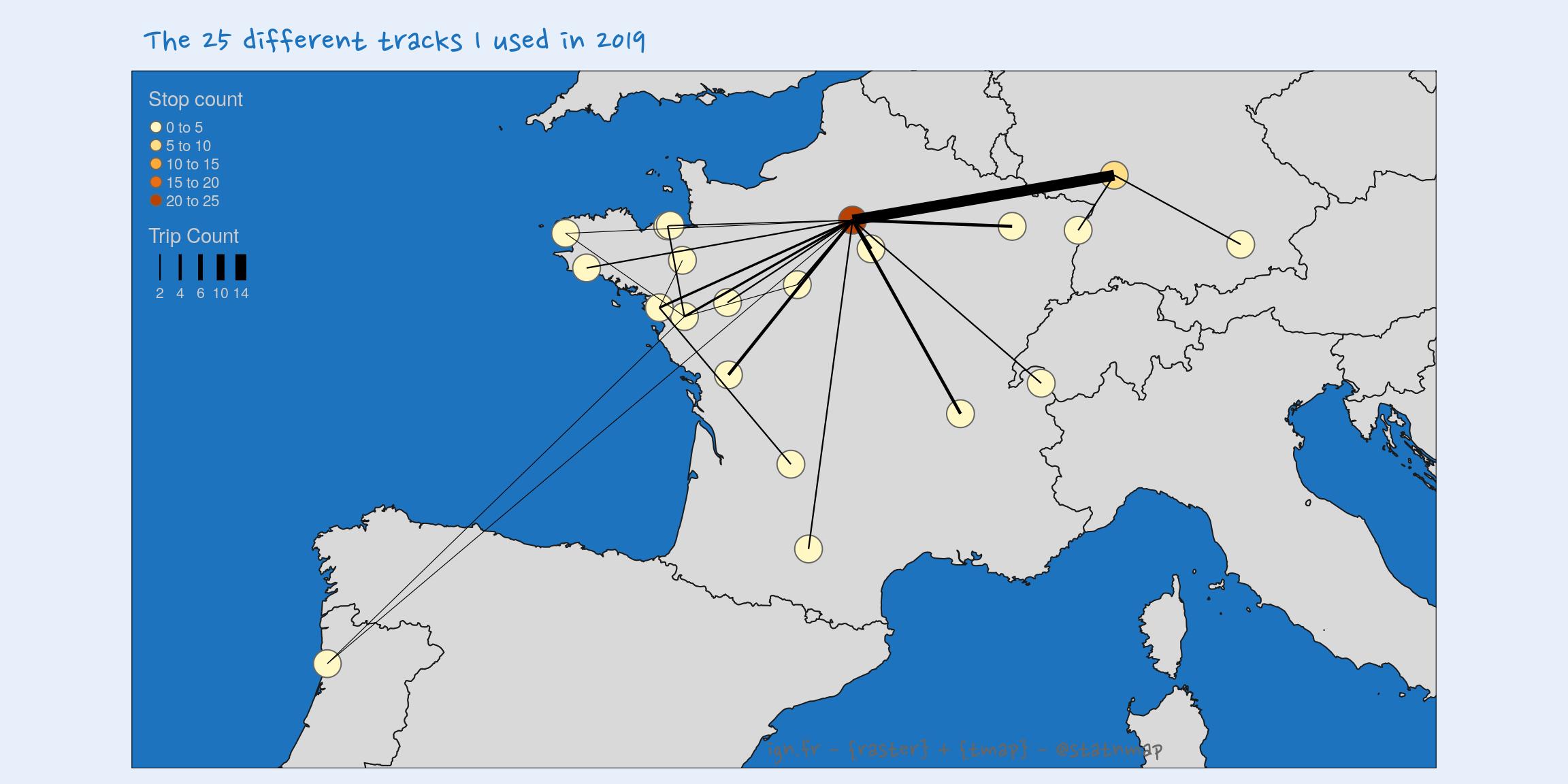

Boundaries: Transform spatial polygons as rasters and use {rayshader}

Let’s try to play with {rayshader}. I use French departement boundaries as walls.

• Transform polygons as lines
• Union all lines into one
• Create a buffer area around lines
• Rasterize buffer polygons
• Rayshade this !
• Transform back as spatial raster
• Plot with {tmap} because this is the {tmap} week!

France_L93_linespolygons <- France_L93 %>% 
  st_simplify(preserveTopology = TRUE, dTolerance = 1000) %>% 
  st_cast("MULTILINESTRING") %>% 
  st_union() %>% 
  st_simplify(preserveTopology = TRUE, dTolerance = 9000) %>% 
  st_buffer(dist = units::set_units(5, "km")) %>% 
  st_sf() %>% 
  mutate(id = 1)

# Transform lines as raster
r <- raster(extent(France_L93), nrow = 500, ncol = 400, 
            crs = st_crs(France_L93)$proj4string,
            vals = 0)
France_L93_lines_r <- rasterize(France_L93_linespolygons, r,
                                background = 0) %>% 
  mask(France_L93)
# mapview::mapview(France_L93_lines_r)

# Let's rayshade this while exagerate walls height
elmat <- raster_to_matrix(France_L93_lines_r * 30000)
elmat_rayed <- elmat %>% 
  ray_shade(zscale = res(r)[1])

# Transform back as a raster
r_shade <- raster::flip(raster(t(elmat_rayed)), direction = "y")
extent(r_shade) <- extent(France_L93_lines_r)
projection(r_shade) <- projection(France_L93_lines_r)
# mapview::mapview(r_shade)

# Plot
palette <- mapview::mapviewGetOption("raster.palette")(20)[1:19]
tm <- tm_shape(r_shade) +
  tm_raster(palette = palette,
            n = 20, style = "quantile", 
            legend.show = FALSE) +
tm_shape(France_L93_linespolygons) +
  tm_fill(col = my_blue, alpha = 0.5) +
tm_credits("ign.fr - {rayshader} + {raster} + {tmap} - @statnmap",
           position = c(0.05, -0.01),
           size = 1.3, fontfamily = "Nanum Pen",
           col = "grey90") +
tm_layout(
    main.title = paste("Internal boundaries?"),
    main.title.color = my_blue,
    main.title.fontfamily = "Nanum Pen",
    main.title.size = 1.75,
    title.fontfamily = "Nanum Pen",
    # Margin to allow legend
    # inner.margins = c(0.15, 0.15, 0.15, 0.15),
    # Colours
    outer.bg.color = c("#E6EFFA"),
    bg.color = my_blue, #"grey60",
    # Legend
    legend.title.color = "grey80",
    legend.text.color = "grey80",
    legend.position = c("left", "top")
  )

tmap_save(tm, filename = file.path(extraWD, "boundaries.jpg"),
          width = 1024, height = 512, units = "px",
          dpi = 100)

tm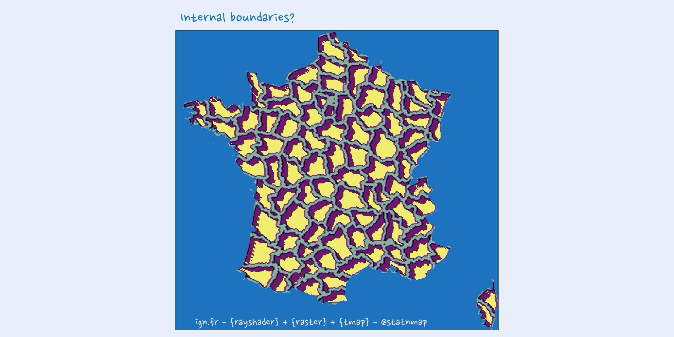

Now that you have seen possibilities of {tmap} to create maps with R, you can read the articles of the others weeks of the challenge:

• Create maps in R with {ggplot2}
• Create maps with a spherical view at the globe scale

As always, code and data are available on https://github.com/statnmap/blog_tips

# Biblio with {chameleon}
tmp_biblio <- tempdir()
attachment::att_from_rmd("2019-11-15-30daymapchallenge-building-maps-2-tmap.Rmd", 
                         inside_rmd = TRUE) %>% 
  chameleon::create_biblio_file(
    out.dir = tmp_biblio, to = "html", edit = FALSE,
    output = "packages")
htmltools::includeMarkdown(file.path(tmp_biblio, "bibliography.html"))

@misc{Roche2019#30Da,
    author = {Rochette Sébastien},
    title = {#30DayMapChallenge: 30 days building maps (2) - tmap},
    url = {https://statnmap.com/2019-11-15-30daymapchallenge-building-maps-2-tmap/},
    year = {2019}
  }