#30DayMapChallenge: 30 days building maps (3) - Earth is spherical

Packages

library(dplyr)
library(sf)
library(rnaturalearth)
library(tmap)
# install.packages("echarts4r")
# remotes::install_github('JohnCoene/echarts4r.assets')
# remotes::install_github('JohnCoene/echarts4r.maps')
library(echarts4r)
library(echarts4r.assets)
library(sp)
# remotes::install_github("JohnCoene/globe4r")
library(globe4r)
library(maps)
library(ggplot2)
library(readr)
library(raster)
library(rgl)
library(geometry)
library(rworldmap)

## Customize
font <- extrafont::choose_font(c("Nanum Pen", "Lato", "sans"))

my_blue <- "#1e73be"
my_theme <- function(font = "Nanum Pen", ...) {
  theme_dark() %+replace%
    theme(
      plot.title = element_text(family = font, 
                                colour = my_blue, size = 18),
      plot.subtitle = element_text(family = font, size = 15),
      # text = element_text(size = 13), #family = font, 
      plot.margin = margin(4, 4, 4, 4),
      plot.background = element_rect(fill = "#f5f5f2", color = NA),
      legend.text = element_text(family = font, size = 10),
      legend.title = element_text(family = font),
      # legend.text = element_text(size = 8),
      legend.background = element_rect(fill = "#f5f5f2"),
      ...
    )
}

Names: Animate a sphere using {tmap}

Let’s find French communes containing “mer/ocean” (= sea) in their name. Note that Maëlle Salmon a similar map with names of rivers and seas in her blog post “French places and a sort of resolution”

# extraWD <- "." # Uncomment for the script to work
communes_L93 <- st_read(file.path(extraWD, "commune_centers.shp"))

communes_mer <- communes_L93 %>% 
  filter(grepl("\\-mer$|\\s+mer$|ocean", tolower(NOM_COM)))

# mapview::mapview(communes_mer)

# https://stackoverflow.com/questions/43207947/whole-earth-polygon-for-world-map-in-ggplot2-and-sf/43278961#43278961
crs <- "+proj=laea +lat_0=52 +lon_0=10 +x_0=4321000 +y_0=3210000 +datum=WGS84 +units=m +no_defs"

world_ne <- ne_countries(scale = 50, type = "countries", returnclass = "sf") %>%
  select(iso_a3, iso_n3, admin, continent)

sphere <- st_graticule(ndiscr = 10000, margin = 10e-6) %>%
  st_transform(crs = crs) %>%
  st_convex_hull() %>%
  summarise(geometry = st_union(geometry))

show_dist <- function(dist, name) {
  
  # Crop World to area around France
  france_large <- world_ne %>% 
    st_crop(communes_mer %>% 
              st_buffer(dist = units::set_units(dist, "km")) %>% 
              st_transform(crs = st_crs(world_ne))) %>% 
        st_transform(crs)
  
  # Plot
  tm <- tm_shape(sphere) +
    tm_fill(col = "#D8F4FF") +
   tm_graticules() +
   tm_shape(france_large, is.master = TRUE) +
    tm_polygons() +
   tm_shape(communes_mer) +
    tm_symbols(col = my_blue) +
   tm_layout() +
    tm_credits("{sf} - {tmap} - @statnmap",
             position = c(0.38, -0.01),
             size = 1.3, fontfamily = "Nanum Pen",
             col = "grey90") +
  tm_layout(
    main.title = "Cities with 'mer' or 'ocean' in names",
    main.title.color = my_blue,
    main.title.fontfamily = "Nanum Pen",
    main.title.size = 1.75,
    title = "Why are there 2 cities named 'mer' in the mainland?",
    title.fontfamily = "Nanum Pen",
    title.bg.color = "white",
    title.bg.alpha = 0.7,
    # Margin to allow legend
    inner.margins = 0,
    # Colours
    outer.bg.color = c("#E6EFFA")#,
    # bg.color = my_blue #"grey60"
  )
  
  tmap_save(tm, filename = file.path(extraWD, "gif", paste0(name, ".jpg")),
          width = 1024, height = 512, units = "px",
          dpi = 100)
}

if (!dir.exists(file.path(extraWD, "gif"))) {
  dir.create(file.path(extraWD, "gif"))
}

seq_dist <- seq(1, 10000, by = 500)
seq_names <- formatC(seq_along(seq_dist), width = 3, flag = 0)
purrr::walk2(seq_dist, seq_names, ~show_dist(.x, .y))

# Create gif
img_frames <- list.files(file.path(extraWD, "gif"),
                         full.names = TRUE)

magick::image_write_gif(magick::image_read(img_frames), 
                          path = file.path(extraWD, "names.gif"), 
                          delay = 3/length(img_frames))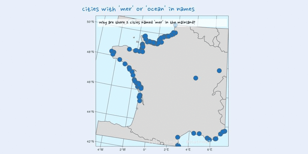

Places: Render an interactive earth globe using {echarts4r}

Let’s map the 7 wonders of the ancient World: Great Pyramid of Giza, Hanging Gardens of Babylon, Temple of Artemis, Statue of Zeus at Olympia, Mausoleum at Halicarnassus, Colossus of Rhodes, and the Lighthouse of Alexandria.
I retrieve coordinates from Wikipedia page “Seven Wonders of the Ancient World”, where there are not all in the same format. For some of the coordinates, I use char2dms() from package {sp}.
For this map, I will use John Coene package {echarts4r} for the first time. I take inspiration in the blog post of Jesus M. Castagnetto (@jmcastagnetto) in “Chart, map and globe showing nuclear explosions (1945-1998)” along with the code from the corresponding Github repository.
I chose to render the output as a gif instead of the interactive html widget of {echarts4r}. I used {htmlwidgets}, {pagedown} and {magick} to create the gif from the HTML page.

# 7 Wonders geographic positions
wonders_wgs84 <- tribble(
  ~id, ~name, ~lat, ~long,
  1, "Giza", as.numeric(char2dms("29d58'45.03\"N")), as.numeric(char2dms("31d08'03.69\"E")),
  2, "Babylon", 32.5355, 44.4275,
  3, "Ephesus", as.numeric(char2dms("37d56'59\"N")), as.numeric(char2dms("27d21'50\"E")),
  4, "Olympia", as.numeric(char2dms("37d38'16.3\"N")), as.numeric(char2dms("21d37'48\"E")),
  5, "Halicarnassus", 37.0379, 27.4241,
  6, "Rhodes", as.numeric(char2dms("36d27'04\"N")), as.numeric(char2dms("28d13'40\"E")),
  7, "Alexandria", as.numeric(char2dms("31d12'50\"N")), as.numeric(char2dms("29d53'08\"E"))
) %>% 
  st_as_sf(coords = c("long", "lat"), crs = 4326, remove = FALSE)

e <- wonders_wgs84 %>% 
  # x-axis (longitude for maps)
  e_charts(long) %>% 
  # globe
  e_globe(
    environment = ea_asset("starfield"),
    base_texture = ea_asset("world topo"),
    height_texture = ea_asset("world topo"),
    globeOuterRadius = 100
  ) %>% 
  # create points, with y-axis column
  e_scatter_3d(lat, id, coord_system = "globe", blendMode = 'lighter') %>% 
  e_visual_map(min = 1, max = 7,
               inRange = list(symbolSize = c(8, 10))) %>% 
  e_toolbox_feature(
    feature = c("saveAsImage", "restore")
  ) %>%
  e_title(
    "Seven Wonders of the Ancient World",
    "Source: @statnmap"
  )


# save as html
htmlwidgets::saveWidget(e, file = file.path(extraWD, "echarts4r-places.html"))

# Create some snapshots of the html
dir_gif <- file.path(extraWD, "gif-globe")
if (!dir.exists(dir_gif)) {dir.create(dir_gif)}
wait_time <- seq(0, 35, by = 2)
for (i in 10:length(wait_time)) {
  pagedown::chrome_print(
    input = file.path(extraWD, "echarts4r-places.html"),
    output = file.path(
      dir_gif,
      paste0("echarts4r-places-", 
             formatC(i, flag = 0, width = 3),
             ".jpeg")
    ),
    format = "jpeg",
    wait = wait_time[i],
    timeout = wait_time[i] + 20)
}

# Create gif
img_frames <- list.files(dir_gif, full.names = TRUE)

magick::image_write_gif(magick::image_read(img_frames), 
                          path = file.path(extraWD, "places.gif"), 
                          delay = 3/length(img_frames))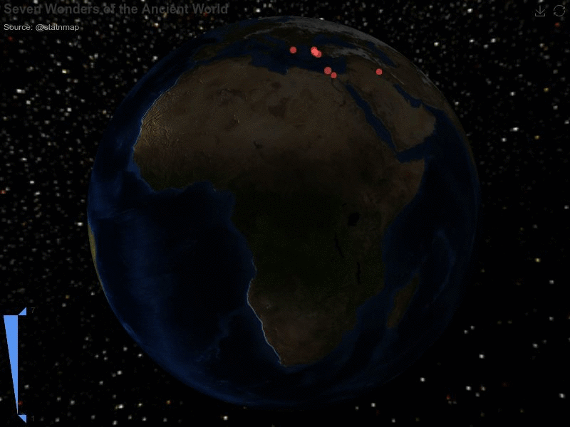

Zones: Divide areas on a sphere using {sf}

I used to leave in Loire-atlantique as you may have understand if you read the first blog post of this map challenge. This department is divided in two parts by the Loire river, and we use to define these two parts, “Nord Loire” and “Sud Loire”. In my point of view, this is also the limit I would put to divide France in North and South. Let’s see where this cuts the World…

• Get hydrography map for France on IGN website
• Get World rivers from {mapdata}
• Find the latitude of this line using {mapview}: around 47.28° if I use the Loire estuary as my reference
• Create a thin polygon layer around the World, defined by this latitude
• Divide the department in two parts
• Divide France in two parts
• Divide the World in two parts
• Plot with {ggplot2}

# France
France_l93 <- st_read(file.path(extraWD, "DEPARTEMENT.shp"))
France_wgs84 <- France_l93 %>% 
  st_transform(crs = 4326)

# Loire river from IGN
Loire_l93 <- st_read(file.path(extraWD, "Loire.shp"))
Loire_wgs84 <- Loire_l93 %>% 
  st_transform(crs = 4326)

# {mapdata} World rivers
rivers_wgs84 <- map('rivers', plot = FALSE) %>% 
  maptools::map2SpatialLines() %>% 
  st_as_sf() %>% 
  st_set_crs(4326) %>% 
  mutate(id = 1:n())

# LA cut ----
# Cut Loire atlantique with river
Loire_buf_l93 <- Loire_l93 %>% 
  st_buffer(dist = units::set_units(1500, "m"))

LA_cut_l93 <- France_l93 %>% 
  filter(CODE_DEPT == 44) %>%  
  st_difference(Loire_buf_l93) %>% 
  st_cast("POLYGON") %>% 
  mutate(id = 1:n())

# mapview::mapview(France_44_inter)
g1 <- ggplot() +
  geom_sf(data = LA_cut_l93, aes(fill = as.character(id))) +
  guides(fill = FALSE) +
  theme(axis.text = element_blank(),
        axis.ticks = element_blank())

# France cut ----
# Find limit
# mapview::mapview(rivers_wgs84)
lat_limit <- 47.28

# Create line to separate North-South
north_line_fr <- matrix(
  c(-5, lat_limit, 
    10, lat_limit),
  ncol = 2, byrow = TRUE
)
line_north_fr_wgs84 <- st_linestring(north_line_fr) %>% 
  st_sample(50) %>% 
  st_cast("LINESTRING") %>% 
  st_sfc(crs = 4326) 

line_north_fr_buf_wgs84 <- line_north_fr_wgs84 %>% 
  st_buffer(dist = 0.01)
  # st_buffer(dist = units::set_units(1500, "m"))

# Cut France in 2 parts
Fr_cut_wgs84 <- France_wgs84 %>% 
  st_union() %>% 
  st_difference(line_north_fr_buf_wgs84) %>% 
  st_cast("POLYGON") %>% 
  st_sf() %>% 
  mutate(id = sample(1:n()))

g2 <- ggplot() +
  geom_sf(data = Fr_cut_wgs84, aes(fill = as.character(id))) +
  geom_sf(data = line_north_fr_buf_wgs84, fill = "red") +
  coord_sf(crs = 2154) +
  guides(fill = FALSE) +
  theme(axis.text = element_blank(),
        axis.ticks = element_blank())

# World cut ----
crs <- "+proj=laea +lat_0=52 +lon_0=10 +x_0=4321000 +y_0=3210000 +datum=WGS84 +units=m +no_defs"

# Get World
world_ne <- rnaturalearth::ne_countries(returnclass = "sf")

# Create line to separate North-South
north_line <- matrix(
  c(-180, lat_limit, 
    180, lat_limit),
  ncol = 2, byrow = TRUE
)
line_north_wgs84 <- st_linestring(north_line) %>% 
  st_sample(300) %>% 
  st_cast("LINESTRING") %>% 
  st_sfc(crs = 4326) 
line_north_buf_wgs84 <- line_north_wgs84 %>% 
  st_buffer(dist = 0.01)

# Cut World in 2 parts
World_cut_wgs84 <- world_ne %>% 
  st_union() %>% 
  st_difference(line_north_buf_wgs84) %>% 
  st_cast("POLYGON") %>% 
  st_sf() %>% 
  mutate(id = sample(1:n()))

g3 <- ggplot() +
  geom_sf(data = World_cut_wgs84, aes(fill = as.character(id))) +
  geom_sf(data = line_north_buf_wgs84, colour = "red") +
  coord_sf(crs = crs) +
  guides(fill = FALSE)


p <- cowplot::plot_grid(
  g1, g2, g3, nrow = 1,
  labels = "What is North really?", 
  label_fontfamily = "Nanum Pen",
  label_colour = my_blue, label_size = 50)

jpeg(filename = file.path(extraWD, "zones.jpg"),
     width = 1024, height = 512, units = "px", pointsize = 12,
     quality = 75
)
p
dev.off()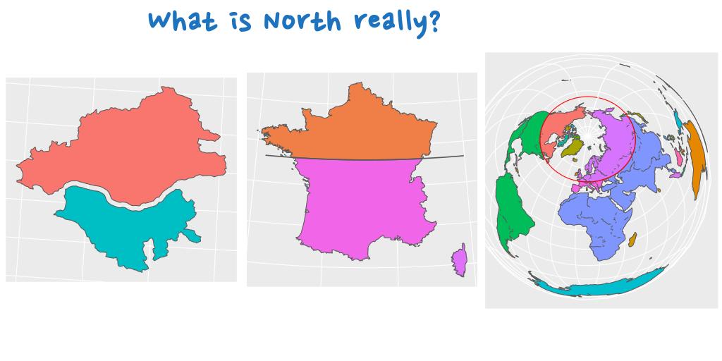

Globe: Create an interactive Earth globe using {globe4r}

Is there a better way to create a globe than using “globe.js”? Let’s quickly play with John Coene {globe4r} package.
My computer has suffered a little too much with this interactive map. So I took a screenshot to avoid hurting your computer when opening this blog post. Who do you thank?

# France
France_l93 <- st_read(file.path(extraWD, "DEPARTEMENT.shp"))
France_wgs84 <- France_l93 %>% 
  st_transform(crs = 4326)

# Create globe
create_globe() %>% 
globe_choropleth(
  data = France_wgs84,
  coords(
    polygon = CODE_REG,
    cap_color = CODE_REG
  ))

# convert to JSON
india_geojson <- geojsonio::geojson_list(France_wgs84)

regions <- india_geojson$features %>% 
  purrr::map("properties") %>% 
  purrr::map("CODE_REG") %>% 
  unlist()

mock_data <- data.frame(
  CODE_REG = regions,
  value = as.numeric(as.character(regions))
)

globe <- create_globe() %>% 
  globe_choropleth(
    data = mock_data,
    coords(
      polygon = CODE_REG,
      cap_color = value,
      altitude = value
    ),
    polygons = india_geojson
  ) %>% 
  globe_pov(47, 2, 0.75) %>% 
  scale_choropleth_cap_color(
    palette = scales::viridis_pal()(5)) %>% 
  scale_choropleth_altitude(max = 0.1) %>%
  show_graticules()
 
# save as html
htmlwidgets::saveWidget(globe, file = file.path(extraWD, "globe4r-globe.html"))

# Print a snapshot - To long to render
# pagedown::chrome_print(
#   input = file.path(extraWD, "globe4r-globe.html"),
#   output = file.path(extraWD,"globe4r-globe.jpeg"),
#   format = "jpeg",
#   wait = 10,
#   timeout = 60)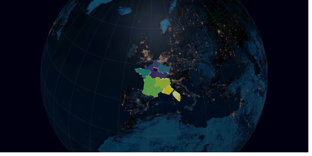

Urban: Create globe view with inset on {ggplot2}

During this challenge, I showed some maps like the distribution of bars in France that are likely to be correlated with the distribution of the population. Today is time to directly show this map of population.
In the dataset world.cities of {maps}, only cities upper than 40000 inhabitants are represented, along with all capital cities of any population size (and some other smaller towns). What looks like France if we separate cities with this 40000 inhabitants limit?

# France data
communes_L93 <- st_read(file.path(extraWD, "commune_centers.shp"))
communes_big_L93 <- communes_L93 %>% 
  mutate(big = if_else(POPULATION >= 40000, TRUE, FALSE))

# World crs ----
crs <- "+proj=laea +lat_0=52 +lon_0=10 +x_0=4321000 +y_0=3210000 +datum=WGS84 +units=m +no_defs"

g1 <- ggplot() + 
  geom_sf(data = communes_big_L93,
          aes(colour = big, size = POPULATION), 
              show.legend = "point") +
  # scale_size_continuous(trans = "log10") +
  scale_size(range = c(0, 4)) +
  scale_colour_viridis_d(name = "Big cities?") +
    labs(
    title = "French cities population",
    subtitle = "Where are big cities (>=40000 inh.)?",
    caption = "ggplot2 - @statnmap - source: ign.fr",
    x = NULL, y = NULL,
    fill = "Number"
  ) +
  coord_sf(crs = 2154) +
  my_theme()

ggsave(plot = g, filename = file.path(extraWD, "urban.jpg"),
       width = 20, height = 10, units = "cm",
       dpi = 200)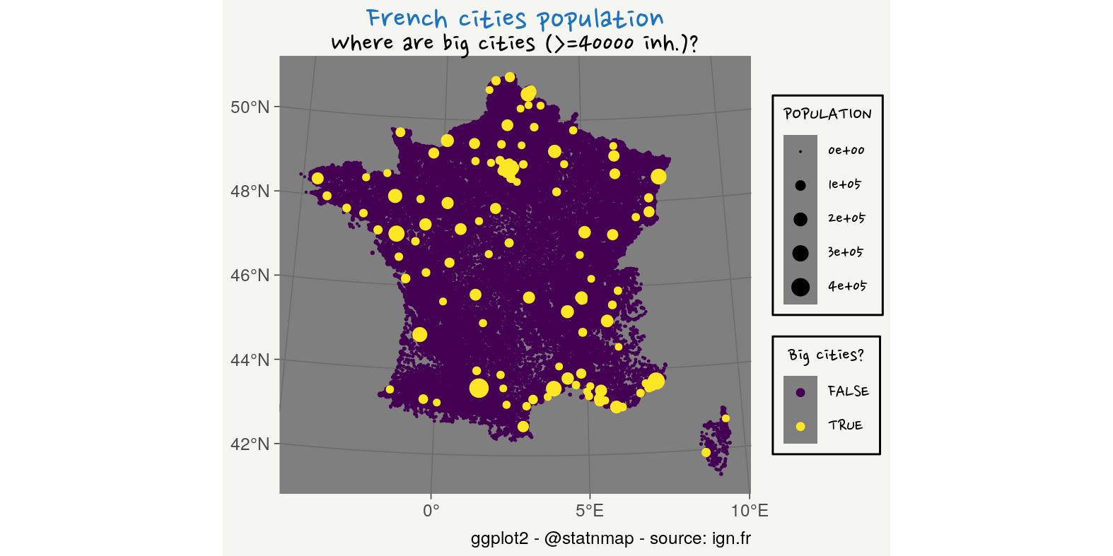

Let’s have a look at France situation in the middle of the World.

# World data
data(world.cities)

w_cities <- world.cities %>% 
  st_as_sf(coords = c("long", "lat"), crs = 4326) %>% 
  rename(POPULATION = pop) %>% 
  mutate(big = if_else(POPULATION >= 40000, TRUE, FALSE))

# Ocean as blue
graticule <- st_graticule(ndiscr = 10000, margin = 10e-6) %>%
  st_transform(crs = crs) 

sphere <- st_graticule(ndiscr = 10000, margin = 10e-6) %>%
  st_transform(crs = crs) %>%
  st_convex_hull() %>%
  summarise(geometry = st_union(geometry))

# France inset
g1 <- ggplot() + 
  geom_sf(data = communes_big_L93,
          aes(colour = big, size = POPULATION), 
              show.legend = "point") +
  # scale_size_continuous(trans = "log10") +
  scale_size(range = c(0, 2)) +
  scale_colour_viridis_d(name = "Big cities?") +
  guides(size = FALSE, colour = FALSE) +
  labs(x = NULL, y = NULL) +
  theme(
    axis.title = element_blank(),
    axis.text = element_blank(),
    axis.ticks = element_blank(),
    panel.background = element_rect(fill = my_blue),
    plot.margin = margin(0,0,0,0)
  )

# World
g2 <- ggplot() + 
  geom_sf(data = sphere, fill = my_blue) +
  geom_sf(data = graticule, size = 0.1) +
  geom_sf(data = w_cities, aes(colour = big, size = POPULATION), 
              show.legend = "point") +
  geom_sf(data = communes_big_L93,
          aes(colour = big, size = POPULATION), 
              show.legend = "point") +
  # scale_size_continuous(trans = "log10") +
  scale_size(range = c(0, 2)) +
  scale_colour_viridis_d(name = "Big cities?") +
    labs(
    title = "World cities population",
    subtitle = "Where are big cities (>=40000 inh.)?",
    caption = "ggplot2 - @statnmap - source: ign.fr",
    x = NULL, y = NULL,
    fill = "Number"
  ) +
  coord_sf(crs = crs) +
  my_theme() +
  # 
  # ggplot() +
  # geom_sf(data = sphere, fill = my_blue) +
  # coord_sf(crs = crs) +
  annotation_custom(
    grob = ggplotGrob(g1),
    xmin = 9e6, xmax = Inf, ymin = -Inf, ymax = 0)

ggsave(plot = g2, filename = file.path(extraWD, "urban_world.jpg"),
       width = 20, height = 10, units = "cm",
       dpi = 200)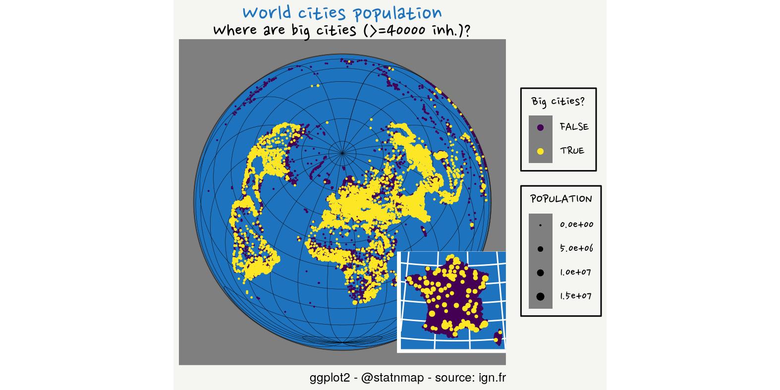

Rural: Create an animated zoom of the Earth globe using {tmap}

I found a dataset of French cities where there is a Protected/Controlled Origin Appelation and a list of all PAO/CAO cheese in a PDF on the INAO website

• Clean datasets with {thinkr}
• Merge with table of PAO/CAO cheese names
• Merge with map of cities centers
  • Merge is not perfect because some cities ID (INSEE_COM) are not all identical in both databases. Thus, I completed with a merge on the name. Some cities are still missing coordinates.

# Cities centers
communes_L93 <- st_read(file.path(extraWD, "commune_centers.shp"))

# Cities with AOP
data_aop <- read_csv2(file.path(extraWD, "2019-11-05-comagri-communes-aires-ao.csv"), locale = locale(encoding = "latin1")) %>% 
  mutate(AOP = thinkr::clean_vec(`Aire géographique`, unique = FALSE))

# AOP for Cheese
names_cheese <- read_csv(file.path(extraWD, "Fromages_fr.csv")) %>% 
  mutate(AOP = thinkr::clean_vec(Fromages, unique = FALSE))

# Filter only cheese names
data_ao_cheese <- data_aop %>% 
  inner_join(names_cheese)

data_ao_cheese_L93 <- communes_L93 %>% 
  right_join(data_ao_cheese, by = c("INSEE_COM" = "CI"))

# Remove empty
data_ao_cheese_insee_L93 <- data_ao_cheese_L93 %>% 
  filter(!st_is_empty(.))

# Get empty and merge with name
data_ao_cheese_empty <- data_ao_cheese %>% 
  anti_join(data_ao_cheese_insee_L93, by = c("CI" = "INSEE_COM")) %>% 
  mutate(COM = toupper(Commune)) 

data_ao_cheese_name_L93 <- communes_L93 %>% 
  right_join(data_ao_cheese_empty, by = c("NOM_COM" = "COM")) %>% 
  filter(!st_is_empty(.)) %>% 
  select(-CI)

# Merge insee + name
data_ao_cheese_complete_l93 <- data_ao_cheese_insee_L93 %>% 
  rbind(data_ao_cheese_name_L93)

# Some still do not have coords  

tm_shape(data_ao_cheese_complete_l93) +
  tm_symbols(col = my_blue, size = 0.1, shape = 20)

# Map
crs <- "+proj=laea +lat_0=52 +lon_0=10 +x_0=4321000 +y_0=3210000 +datum=WGS84 +units=m +no_defs"

# Transformation requires st_make_valid()
world_ne <- ne_countries(scale = 50, type = "countries", returnclass = "sf") %>%
  select(iso_a3, iso_n3, admin, continent) %>% 
  st_transform(crs = crs) %>%
  lwgeom::st_make_valid() 

# Background
graticule <- st_graticule(ndiscr = 10000, margin = 10e-6) %>%
  st_transform(crs = crs)
sphere <- graticule %>%
  st_convex_hull() %>%
  summarise(geometry = st_union(geometry))

# Function
show_dist <- function(
  world_ne,
  dist, name, points, 
  crs = "+proj=laea +lat_0=52 +lon_0=10 +x_0=4321000 +y_0=3210000 +datum=WGS84 +units=m +no_defs") {
  
  points <- st_transform(points, crs)
  
  # Get bbox buffer
  bbox_pt_buffer <- points %>% 
    st_bbox() %>%
    st_as_sfc() %>% 
    st_transform(crs = st_crs(world_ne)) %>% 
    st_buffer(dist = units::set_units(dist, "km"))
  
  # Crop World to area around France
  france_large <- world_ne %>% 
    st_crop(bbox_pt_buffer) %>% 
    st_transform(crs)

  # Plot
  tm <- tm_shape(sphere) +
    tm_fill(col = "#D8F4FF") +
   # tm_graticules() +
    tm_shape(graticule) +
    tm_lines(col = "grey30", lwd = 0.5) +
   tm_shape(france_large, is.master = TRUE) +
    tm_polygons() +
   tm_shape(points) +
    tm_symbols(col = my_blue, size = 0.1, shape = 20) +
   tm_layout() +
    tm_credits("{sf} - {tmap} - @statnmap",
             position = c(0.38, -0.01),
             size = 1.3, fontfamily = "Nanum Pen",
             col = "grey90") +
  tm_layout(
    main.title = "French cities where there is AOP cheese",
    main.title.color = my_blue,
    main.title.fontfamily = "Nanum Pen",
    main.title.size = 1.75,
    title = "What would be France without cheese?",
    title.fontfamily = "Nanum Pen",
    title.bg.color = "white",
    title.bg.alpha = 0.7,
    # Margin to allow legend
    inner.margins = 0,
    outer.margins = c(0.01, 0.17, 0.01, 0.17),
    # Colours
    outer.bg.color = c("#E6EFFA")#,
    # bg.color = my_blue #"grey60"
  )
  
  tmap_save(tm, filename = file.path(extraWD, "gif-rural", paste0(name, ".jpg")),
          width = 1024, height = 512, units = "px",
          dpi = 100)
}

# Create each frame
# show_dist(world_ne = world_ne,
#           dist = 500,
#           name = "001",
#           points = data_ao_cheese_complete_l93)

if (!dir.exists(file.path(extraWD, "gif-rural"))) {
  dir.create(file.path(extraWD, "gif-rural"))
}

seq_dist <- seq(1, 15000, by = 500)
seq_names <- formatC(seq_along(seq_dist), width = 3, flag = 0)
purrr::walk2(
  seq_dist, seq_names,
  ~show_dist(dist = .x,
             name = .y,
             world_ne = world_ne,
             points = data_ao_cheese_complete_l93))

# Create gif
img_frames <- list.files(
  file.path(extraWD, "gif-rural"),
  full.names = TRUE)

magick::image_write_gif(
  magick::image_read(img_frames), 
  path = file.path(extraWD, "rural.gif"), 
  delay = 3/length(img_frames))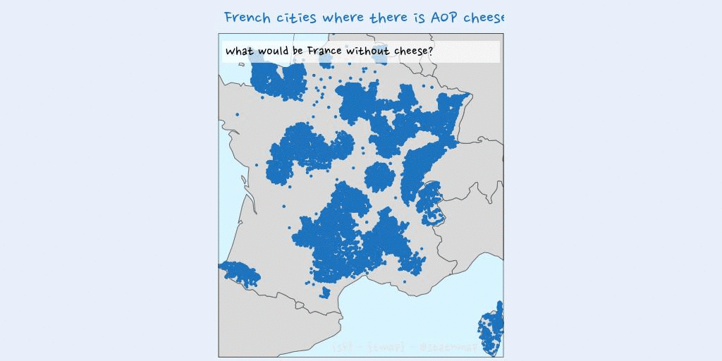

Environment: Plot raster on a sphere with {rgl}

We download data from Worldclim with function getData of package {raster}. In this map, I will show a environment variable: Annual Precipitation (BIO12).

• Download dataset
• Reduce resolution
• Plot on an 3D sphere following my blog post on Spatial interpolation on Earth as a 3D sphere using {GeoDist}, Constrained distance calculation and associated geotools and {rgl}

prec <- raster::getData("worldclim", var = "bio", 
                path = extraWD, res  = 10)

bio12 <- raster(prec, 12) %>% 
  raster::aggregate(fact = 5, fun = sum)
# plot(bio12)

# Transform as cartesian coordinates
r.cart <- data.frame(GeoDist::sph2car(coordinates(bio12)))
# Triangulate entire globe directly with geometry ----
tri3d <- geometry::convhulln(r.cart)
r.cart.tri <- r.cart[t(tri3d), ] %>%
  mutate(n = c(t(tri3d)))

# Define a vector of colors for predictions
n.break <- 20
colors <- alpha(colorRampPalette(c("#ffffcc", my_blue))(n.break), .4)
brk <- seq(minValue(bio12), maxValue(bio12), len = n.break + 1)
pred.col <- colors[as.numeric(as.character(values(
  raster::cut(bio12, breaks = brk, include.lowest = TRUE))))]

# Print in 3d
triangles3d(r.cart.tri$x,
            r.cart.tri$y,
            r.cart.tri$z,
            col = pred.col[r.cart.tri$n],
            alpha = 0.9,
            specular = "black")
# Black background
rgl.bg(color = c("black"))
# Add Earth rotation axe
segments3d(x = c(0,0),
           y = c(0,0),
           z = c(min(r.cart.tri$z)*1.2, 
                 max(r.cart.tri$z)*1.2),
           col = "white",
           lwd = 2)

# Map world on the 3d sphere ----
data(countriesCoarse)

for (i in 1:nrow(countriesCoarse)) { # i <- 1
  Pols <- countriesCoarse@polygons[[i]]  
  for (j in 1:length(Pols)) { # j <- 1
    lines3d(data.frame(GeoDist::sph2car(
      countriesCoarse@polygons[[i]]@Polygons[[j]]@coords
    )), col = "white", lwd = 2)
  }
}

# Rotate and save as gif
# extraWD: directory where to save img of rotation
nb.img <- 45
angle.rad <- seq(0, 2*pi, length.out = nb.img)
# NorthPole on top, Europe-Africa in front.
uM0 <- rotationMatrix(-pi/2, 1, 0, 0) %>%
  transform3d(rotationMatrix(-2, 0, 0, 1)) %>%
  transform3d(rotationMatrix(-pi/12, 1, 0, 0))
# Change viewpoint
rgl.viewpoint(theta = 0, phi = 0, fov = 0, zoom = 0.7,
              userMatrix = uM0)

if (!dir.exists(file.path(extraWD, "gif-envt"))) {
  dir.create(file.path(extraWD, "gif-envt"))
}
for (i in 1:nb.img) {
  # Calculate matrix rotation
  uMi <- transform3d(uM0, rotationMatrix(-angle.rad[i], 0, 0, 1))
  # Change viewpoint
  rgl.viewpoint(theta = 0, phi = 0, fov = 0, zoom = 0.7,
                userMatrix = uMi)
  # Save image
  filename <- file.path(extraWD, "gif-envt", paste0(formatC(i, digits = 1, flag = "0"), ".png"))
  rgl.snapshot(filename)    
}
# Create gif
# Create gif
img_frames <- list.files(
  file.path(extraWD, "gif-envt"),
  full.names = TRUE)

magick::image_write_gif(
  magick::image_read(img_frames), 
  path = file.path(extraWD, "envt.gif"), 
  delay = 3/length(img_frames))

Now that you have seen different possibilities to create maps with a globe view with R, you can read the articles of the others weeks of the challenge:

• Create maps in R with {ggplot2}
• Create maps in R with {tmap}

As always, code and data are available on https://github.com/statnmap/blog_tips

# Biblio with {chameleon}
tmp_biblio <- tempdir()
attachment::att_from_rmd("2019-11-22-30daymapchallenge-building-maps-3-earth-is-sphere.Rmd", inside_rmd = TRUE) %>% 
  chameleon::create_biblio_file(
    out.dir = tmp_biblio, to = "html", edit = FALSE,
    output = "packages")
htmltools::includeMarkdown(file.path(tmp_biblio, "bibliography.html"))

@misc{Roche2019#30Da,
    author = {Rochette Sébastien},
    title = {#30DayMapChallenge: 30 days building maps (3) - Earth is spherical},
    url = {https://statnmap.com/2019-11-22-30daymapchallenge-building-maps-3-earth-is-sphere/},
    year = {2019}
  }