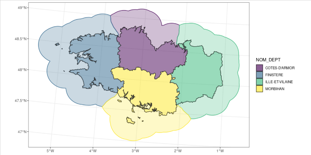
A few weeks ago, Christina Buelow asked on Twitter how she could create the polygons of coastal waters using the land polygons, and making sure there is no overlap in buffer areas. This would make it possible to know which land area is closest to any place in the sea. Let’s explore what solution emerged from the discussions.
TL;DR
- Install {cartomisc} package from GitHub
- Download some data
# Define where to save the dataset
extraWD <- tempdir()
# Get some data available to anyone
if (!file.exists(file.path(extraWD, "departement.zip"))) {
  githubURL <- "https://github.com/statnmap/blog_tips/raw/master/2018-07-14-introduction-to-mapping-with-sf-and-co/data/departement.zip"
  download.file(githubURL, file.path(extraWD, "departement.zip"))
  unzip(file.path(extraWD, "departement.zip"), exdir = extraWD)
}- Reduce the dataset to a small region
library(sf)
# remotes::install_github("statnmap/cartomisc")
library(cartomisc)
library(dplyr)
library(ggplot2)

departements_l93 <- read_sf(dsn = extraWD, layer = "DEPARTEMENT")

# Reduce dataset
bretagne_l93 <- departements_l93 %>%
filter(NOM_REG == "BRETAGNE")- Calculate the regional buffer area using
regional_seas()
bretagne_regional_2km_l93 <- regional_seas(
  x = bretagne_l93,
  group = "NOM_DEPT",
  dist = units::set_units(30, km), # buffer distance
  density = units::set_units(0.5, 1/km) # density of points (the higher, the more precise the region attribution)
)- Plot the data
ggplot() +
  geom_sf(data = bretagne_regional_2km_l93,
          aes(colour = NOM_DEPT, fill = NOM_DEPT),
          alpha = 0.25) +
  geom_sf(data = bretagne_l93,
          aes(fill = NOM_DEPT),
          colour = "grey20",
          alpha = 0.5) +
  scale_fill_viridis_d() +
  scale_color_viridis_d() +
  theme_bw()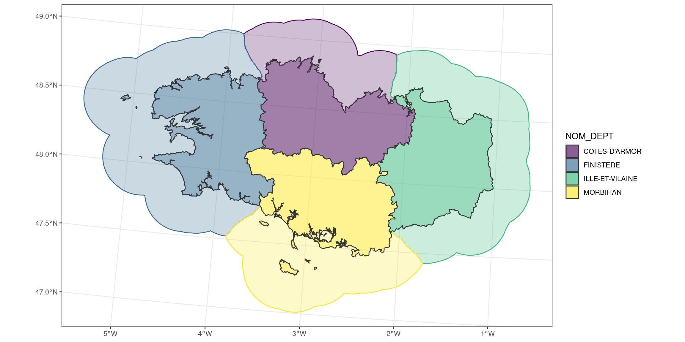
If you want to know the long story, you can continue reading this blog post, otherwise, you have everything you need to start on your own data !
Create buffer area around adjacent polygons
As always when trying to figure out a solution to a specific problem, let’s start with a reproducible example, commonly called “reprex” among R users. This means, we create the minimal code that allows anyone to execute the code, face the same problem and show everything we tested. In the present case, I couldn’t find enough time to reach a solution during the discussions, so I prepared a gist showing what I tried, what point I reached, and more importantly what I plan to achieve.
First, we load some packages
library(sf)
library(ggplot2)
library(dplyr)

my_blue <- "#1e73be"
Then we download some data
# Define where to save the dataset
extraWD <- "."
# Get some data available to anyone
if (!file.exists(file.path(extraWD, "departement.zip"))) {
  githubURL <- "https://github.com/statnmap/blog_tips/raw/master/2018-07-14-introduction-to-mapping-with-sf-and-co/data/departement.zip"
  download.file(githubURL, file.path(extraWD, "departement.zip"))
  unzip(file.path(extraWD, "departement.zip"), exdir = extraWD)
}
I reduce the dataset to better see what I am doing. Here, I filter the Brittany area.
As you can see, there are 4 departments in this region, thus 4 spatial features.
departements_l93 <- read_sf(dsn = extraWD, layer = "DEPARTEMENT")

# Reduce dataset
bretagne_l93 <- departements_l93 %>%
  filter(NOM_REG == "BRETAGNE")

bretagne_l93
## Simple feature collection with 4 features and 11 fields
## Geometry type: MULTIPOLYGON
## Dimension: XY
## Bounding box: xmin: 99217.1 ymin: 6704195 xmax: 400572.3 ymax: 6881964
## Projected CRS: RGF93_Lambert_93
## # A tibble: 4 x 12
## ID_GEOFLA CODE_DEPT NOM_DEPT CODE_CHF NOM_CHF X_CHF_LIEU Y_CHF_LIEU X_CENTROID
## * <chr> <chr> <chr> <chr> <chr> <int> <int> <int>
## 1 DEPARTEM… 35 ILLE-ET… 238 RENNES 351870 6789646 326237
## 2 DEPARTEM… 22 COTES-D… 278 SAINT-… 274947 6839206 260216
## 3 DEPARTEM… 29 FINISTE… 232 QUIMPER 171326 6789950 115669
## 4 DEPARTEM… 56 MORBIHAN 260 VANNES 267889 6744074 256790
## # … with 4 more variables: Y_CENTROID <int>, CODE_REG <chr>, NOM_REG <chr>,
## # geometry <MULTIPOLYGON [m]>Now, I can plot the output of buffer areas around separate polygons.
# Create buffer
bretagne_buffer_l93 <- bretagne_l93 %>%
  st_buffer(
  dist =
    units::set_units(10, km)
)

ggplot() +
  geom_sf(data = bretagne_buffer_l93, fill = my_blue, alpha = 0.2, colour = my_blue) +
  geom_sf(data = bretagne_l93, fill = NA) +
  theme_bw()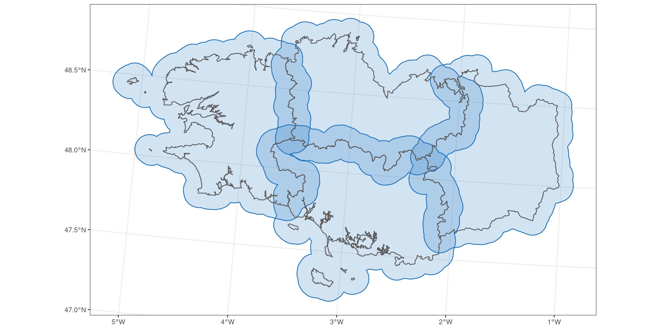
You can see there are overlapping areas.
This is where Voronoï polygons come to help us. From here, I will take some ideas that Christina gathered during her Twitter discussions. Her complete code for coastal buffers is here.
# Create a merged region entity
bretagne_union_l93 <- bretagne_l93 %>%
  summarise()

ggplot() +
  geom_sf(data = bretagne_union_l93, colour = my_blue, fill = NA)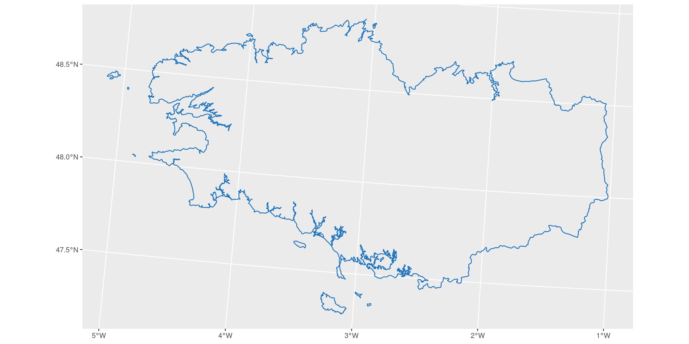
# Create a doughnut for regional seas areas, 30km off coasts
bretagne_seas_l93 <- bretagne_union_l93 %>%
  st_buffer(
    dist = units::set_units(30, km)
  ) %>%
  st_cast()

ggplot() +
  geom_sf(data = bretagne_seas_l93, colour = my_blue, fill = NA)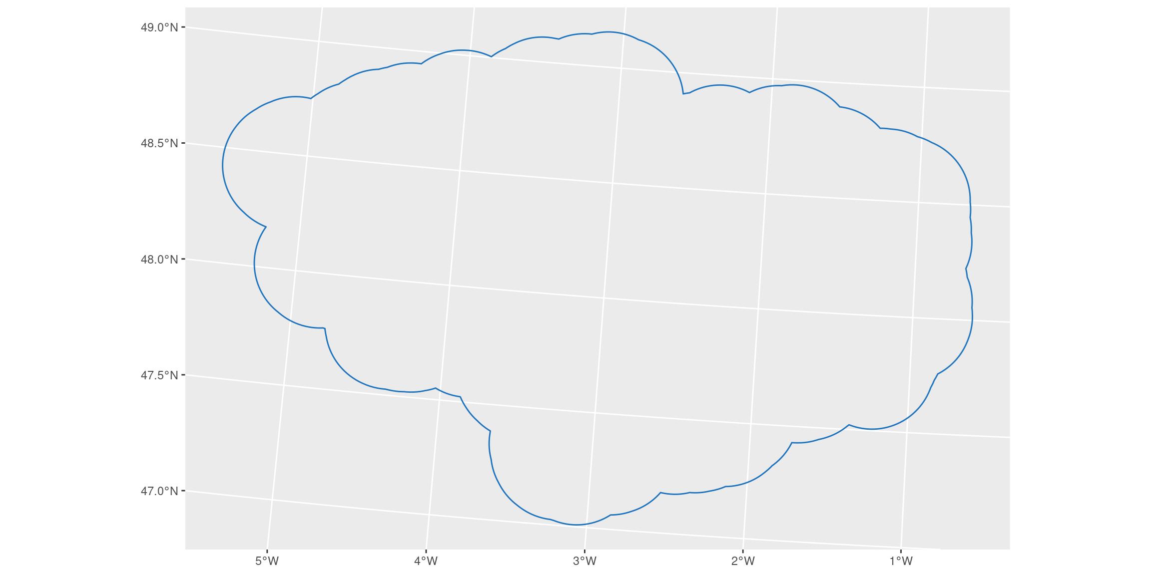
# Remove inside terrestrial parts
bretagne_donut_l93 <- bretagne_seas_l93 %>%
  st_difference(bretagne_union_l93) %>%
  st_cast()

ggplot() +
  geom_sf(data = bretagne_donut_l93, colour = my_blue, fill = my_blue, alpha = 0.2)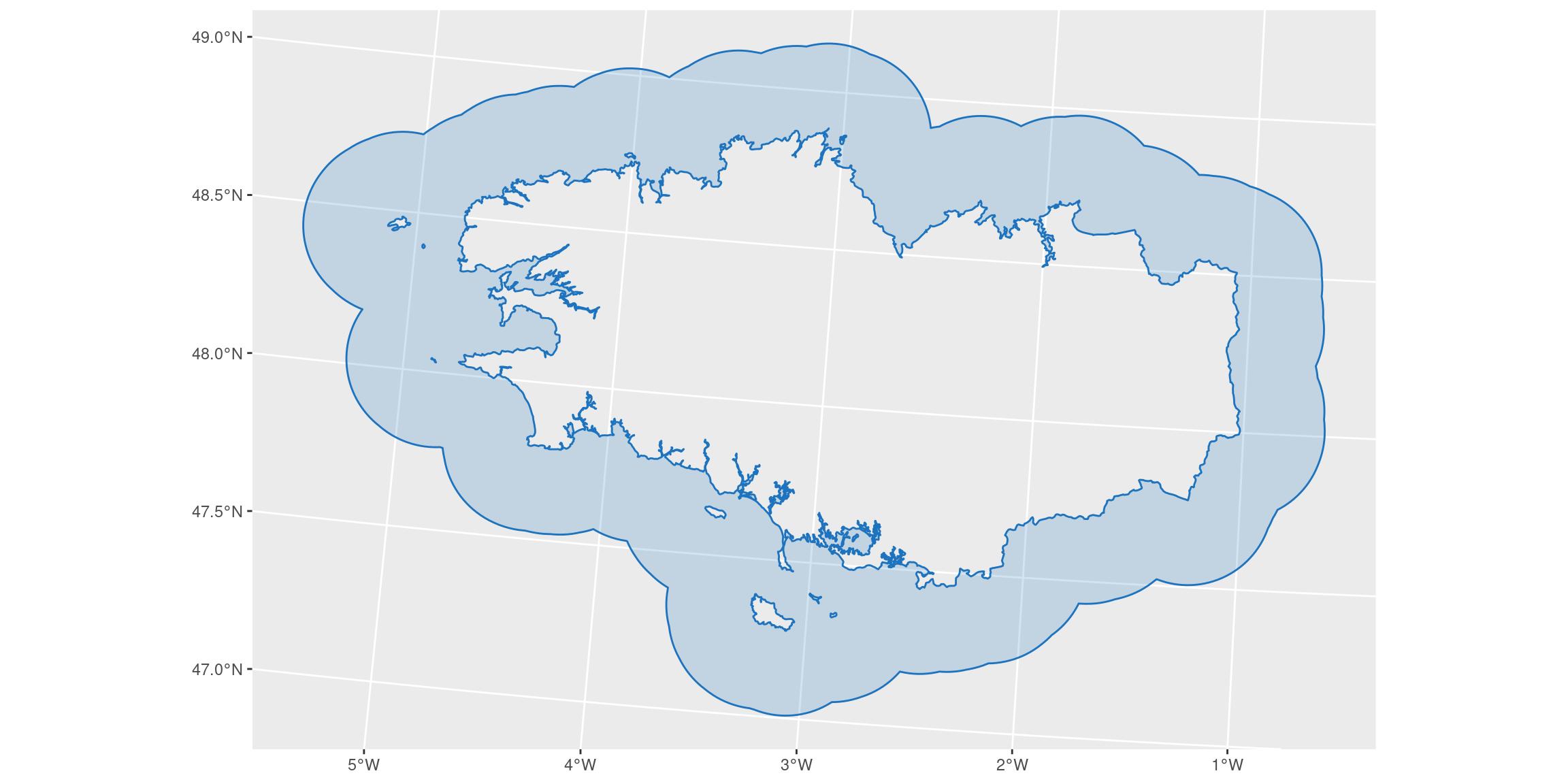
Let’s divide this area in multiples polygons
We use the coastlines as a basis.
# density <- units::set_units(0.1, 1/km)

# First merge everything and transform as lines
bretagne_points_l93 <- bretagne_union_l93 %>%
  # transform polygons as multi-lines
  st_cast("MULTILINESTRING") %>%
  # transform multi-lines as separate unique lines
  st_cast("LINESTRING") %>%
  # transform as points, 0.1 per km (= 1 every 10 km)
  # Choose density according to precision needed
  st_line_sample(density = units::set_units(0.1, 1/km)) %>%
  st_sf() #%>%
  # remove empty geometry (small islands where sample is not possible with this density)
  # filter(!st_is_empty(geometry))

ggplot() +
  geom_sf(data = bretagne_points_l93, colour = my_blue, fill = NA)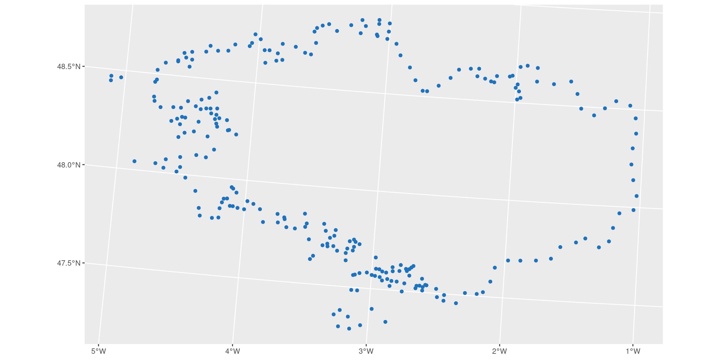
# Create voronoi polygons around points
bretagne_voronoi_l93 <- bretagne_points_l93 %>%
  st_combine() %>%
  st_voronoi() %>%
  st_cast()

ggplot() +
  geom_sf(data = bretagne_voronoi_l93, colour = my_blue, fill = NA)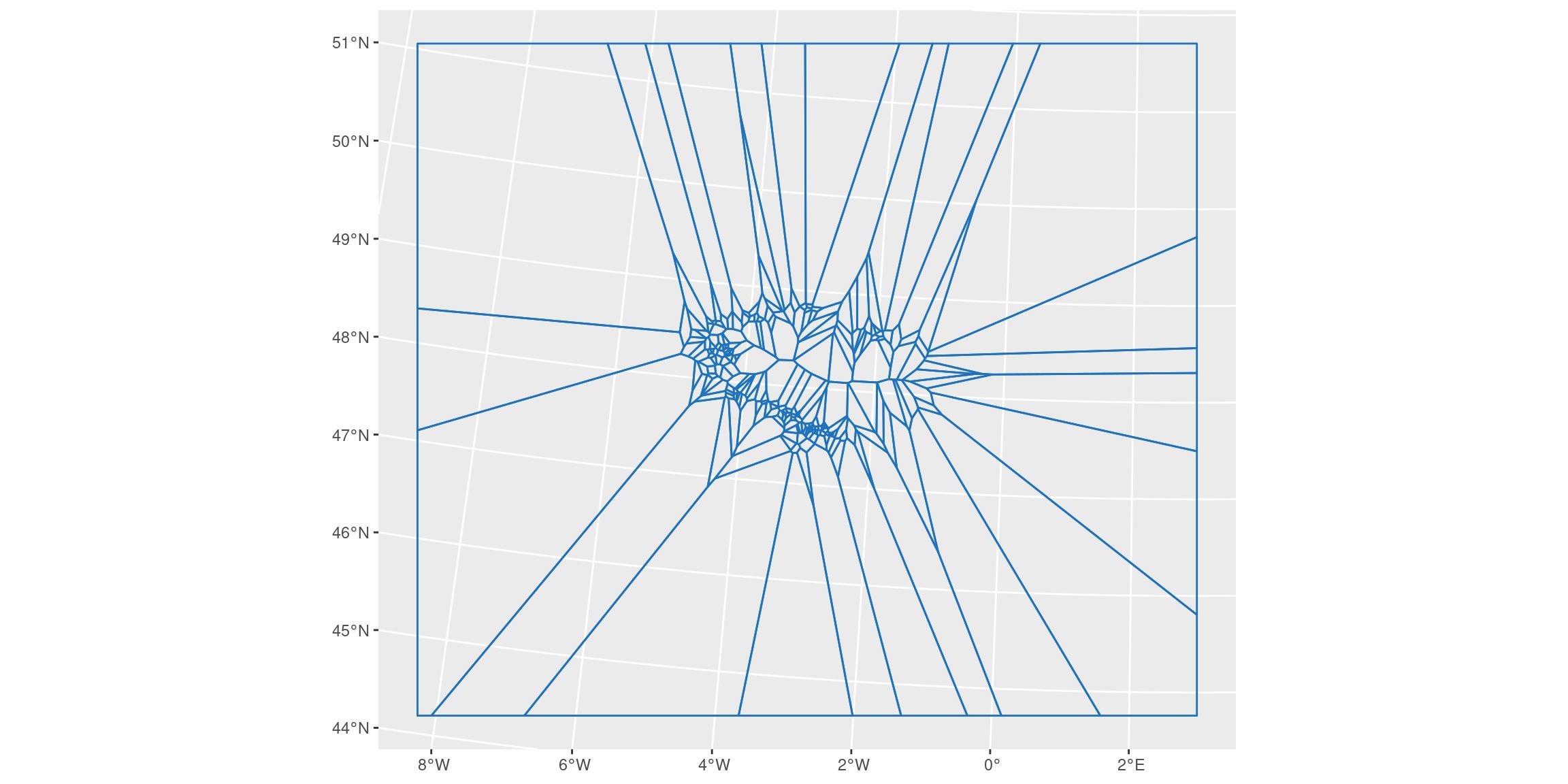
Join voronoi and donut polygon
bretagne_voronoi_donut_l93 <- bretagne_voronoi_l93 %>%
  st_intersection(bretagne_donut_l93) %>%
  st_cast() %>%
  st_sf()

ggplot() +
  geom_sf(data = bretagne_voronoi_donut_l93, colour = my_blue, fill = NA)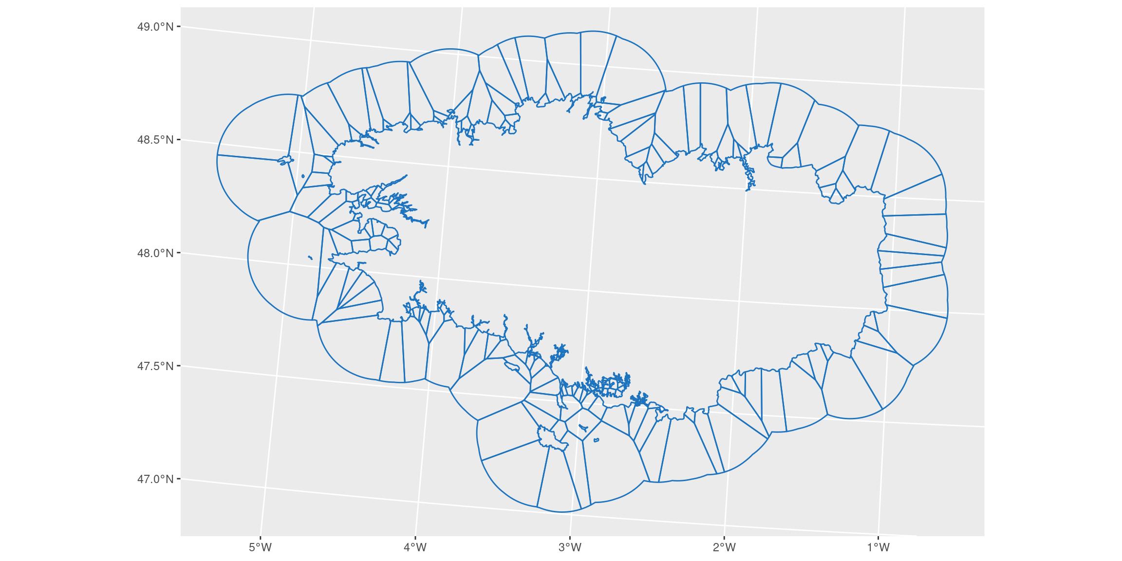
Join voronoi-donut polygons to original dataset to intersect with regions
We realise sort of a left_join based on spatial attributes using st_join(). This will keep the original geometry of our voronoi-donut polygons, while retrieving variables of joined terrestrial dataset when there is intersection.
# Equivalent to left_join
bretagne_vd_region_l93 <- bretagne_voronoi_donut_l93 %>%
  st_join(bretagne_l93)

ggplot() +
  geom_sf(data = bretagne_vd_region_l93,
          aes(colour = NOM_DEPT, fill = NOM_DEPT),
          alpha = 0.25)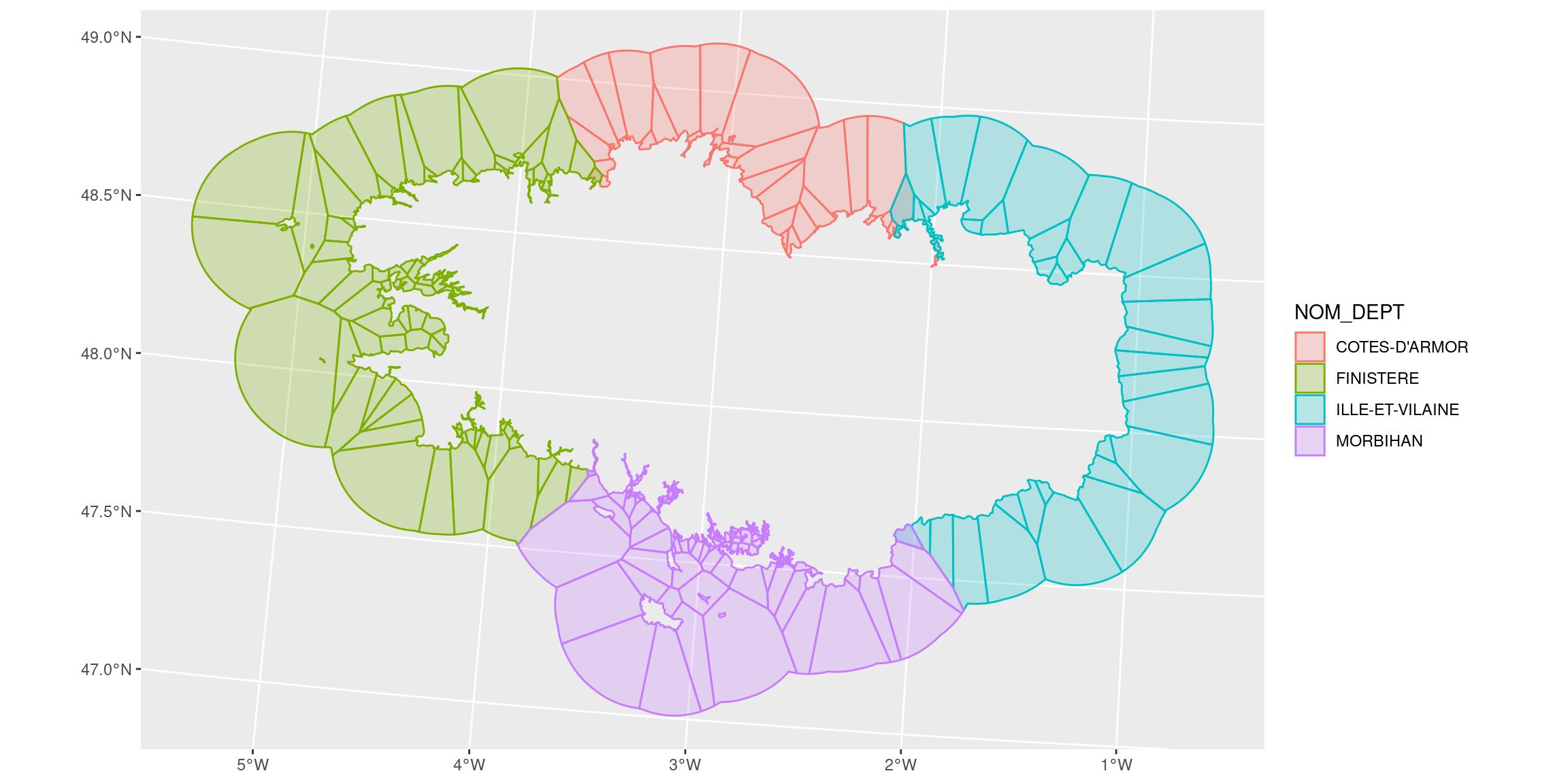
# Interactive view
mapview::mapview(bretagne_vd_region_l93, zcol = "NOM_DEPT")
If we zoom on the map using mapview(), you can see that polygons between two regions sees a double attribution. This is because voronoi intersect with both regions. If you want to reduce the size of the overlapping polygons, you can increase the density of points used to create the voronoi polygons in st_line_sample(). However, we will always have the double attribution. Remember that st_join() works like left_join(). If there are duplicate keys, entities are doubled.
To avoid this, we will have to choose between one region or the other. First, we give a number to the voronoi polygons before joining to be able to identify those that are doubled. Then, we will choose to keep only the first of them in the list. Note that summarise_all does not exists for {sf} objects. I cannot use group_by(id_v) + summarise_all(first) as for classical datasets, neither the new across() function. I use distinct() with parameter keep_all = TRUE so that it keeps all variables with the first entity for each voronoi polygon.
bretagne_vd_region_distinct_l93 <- bretagne_voronoi_donut_l93 %>%
  mutate(id_v = 1:n()) %>%
  st_join(bretagne_l93) %>%
  # group_by(id_v) %>%
  # summarise(across(.cols = everything(), .fns = first)) # Not on {sf}
  # summarise_all(.funs = first) # Not on {sf}
  distinct(id_v, .keep_all = TRUE)

ggplot() +
  geom_sf(data = bretagne_vd_region_distinct_l93,
          aes(colour = NOM_DEPT, fill = NOM_DEPT),
          alpha = 0.25)
# Interactive view
mapview::mapview(bretagne_vd_region_distinct_l93, zcol = "NOM_DEPT")
Join all polygons according to the variable of interest
I can now union polygons.
bretagne_seas_l93 <- bretagne_vd_region_distinct_l93 %>%
  group_by(NOM_DEPT) %>%
  summarise()


ggplot() +
  geom_sf(data = bretagne_seas_l93,
          aes(colour = NOM_DEPT, fill = NOM_DEPT),
          alpha = 0.25) +
  geom_sf(data = bretagne_l93,
          aes(fill = NOM_DEPT),
          colour = "grey20",
          alpha = 0.5)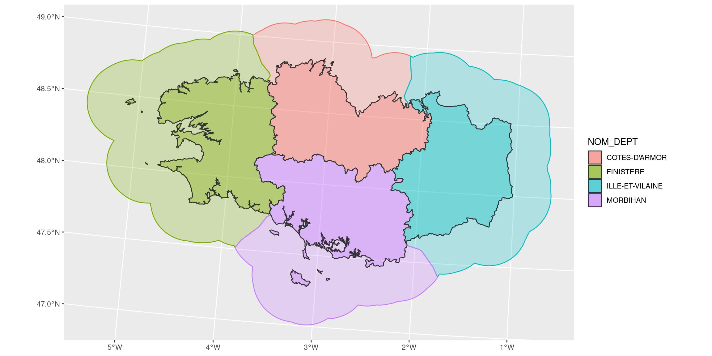
Create buffer areas with attribute of the closest region with {cartomisc}
I cannot let you leave without a function that gathers everything and its application with a higher density of points along the coastlines. The function is written below but is also now avaible with my {cartomisc} package: “Miscellaneous Tools for Spatial Data Manipulation and Analysis”
#' @param x Spatial polygon layer
#' @param group Character. The grouping variable for your subareas
#' @param dist distance from coasts of the buffer area. See ?sf::st_buffer
#' @param density density of points along the coastline
#'
#' @importFrom sf st_buffer st_cast st_difference st_line_sample st_sf st_geometry
#' @importFrom sf st_combine st_voronoi st_intersection st_join
#' @importFrom dplyr summarise mutate distinct group_by_at

regional_seas <- function(x,
                          group,
                          dist = units::set_units(30, km),
                          density = units::set_units(0.1, 1/km)
                          ) {

  # Create a merged region entity
  x_union <- x %>%
    summarise()

  # Create a doughnut for regional seas areas, 30km off coasts
  x_donut <- x_union %>%
    st_buffer(
      dist = dist
    ) %>%
    st_cast() %>%
    # Remove inside terrestrial parts
    st_difference(x_union) %>%
    st_cast()

  # First merge everything and transform as lines
  x_lines <- x_union %>%
    # transform polygons as multi-lines
    st_cast("MULTILINESTRING") %>%
    # transform multi-lines as separate unique lines
    st_cast("LINESTRING")

  # Then as regular points
  x_points <- x_lines %>%
    # transform as points, 0.1 per km (= 1 every 10 km)
    # Choose density according to precision needed
    st_line_sample(density = density) %>%
    st_sf() #%>%
  # remove empty geometry (small islands where sample is not possible with this density)
  # filter(!st_is_empty(geometry))

  if (any(st_is_empty(x_points$geometry))) {
    # Add original islands if empty
    x_lines_multipoints <- x_lines %>%
      st_cast("MULTIPOINT")
    # replace geometry with original lines as points
    st_geometry(x_points)[st_is_empty(x_points$geometry)] <-
      st_geometry(x_lines_multipoints)[st_is_empty(x_points$geometry)]

    x_points <- x_points %>% st_cast()

    warning("There were empty geometries after sampling points along coastlines. ",
            "'density' was probably not big enough for some isolated polygons. ",
            "They have been reinstated with their original resolution")
  }

  # Create voronoi polygons around points
  x_vd_region_distinct <- x_points %>%
    st_combine() %>%
    st_voronoi() %>%
    st_cast() %>%
    st_intersection(x_donut) %>%
    st_cast() %>%
    st_sf() %>%
    mutate(id_v = 1:n()) %>%
    st_join(x) %>%
    # group_by(id_v) %>%
    # summarise(across(.cols = everything(), .fns = first)) # Not on {sf}
    # summarise_all(.funs = first) # Not on {sf}
    distinct(id_v, .keep_all = TRUE)

  # group by variable
  if (!missing(group)) {
    x_seas <- x_vd_region_distinct %>%
      group_by_at(group) %>%
      summarise()

    return(x_seas)
  }

  return(x_vd_region_distinct)
}
Apply the function to our area with a 2km resolution (density = 0.5 points per km)
# remotes::install_github("statnmap/cartomisc")
library(cartomisc)

bretagne_regional_2km_l93 <- regional_seas(
  x = bretagne_l93,
  group = "NOM_DEPT",
  density = units::set_units(0.5, 1/km)
)

# Plot
ggplot() +
  geom_sf(data = bretagne_regional_2km_l93,
          aes(colour = NOM_DEPT, fill = NOM_DEPT),
          alpha = 0.25) +
  geom_sf(data = bretagne_l93,
          aes(fill = NOM_DEPT),
          colour = "grey20",
          alpha = 0.5) +
  scale_fill_viridis_d() +
  scale_color_viridis_d() +
  theme_bw()
Test {cartomisc} and report
You can try this function on Github in {cartomisc} package with your own datasets. If you want to improve it or if you face some problems with your specific spatial data, feel free to open a pull request or an issue.
As always, code and data are available on https://github.com/statnmap/blog_tips
Citation:
For attribution, please cite this work as:
Rochette Sébastien. (2020, Aug. 19). "Buffer areas for nearest neighbours or national marine areas delineation". Retrieved from https://statnmap.com/2020-07-31-buffer-area-for-nearest-neighbour/.
BibTex citation:
@misc{Roche2020Buffe,
    author = {Rochette Sébastien},
    title = {Buffer areas for nearest neighbours or national marine areas delineation},
    url = {https://statnmap.com/2020-07-31-buffer-area-for-nearest-neighbour/},
    year = {2020}
  }

