Analyse de sensibilité de la matrice de communauté inverse

Publications liées

Lassalle Geraldine, Bourdaud Pierre, Saint-Beat Blanche, Rochette Sebastien, Niquil Nathalie (2014). A toolbox to evaluate data reliability for whole-ecosystem models: Application on the Bay of Biscay continental shelf food-web model. Ecological Modelling, 285, 13-21. Publisher’s official version : http://dx.doi.org/10.1016/j.ecolmodel.2014.04.002 , Open Access version : http://archimer.ifremer.fr/doc/00188/29969/

Rochette Sébastien, Lobry Jeremy, Lepage Mario, Boet Philippe (2009). Dealing with uncertainty in qualitative models with a semi-quantitative approach based on simulations. Application to the Gironde estuarine food web (France). Ecological Modelling, 220, 122-132. http://dx.doi.org/10.1016/j.ecolmodel.2008.09.017 The associated presentation:
Inverse Matrix: an easy tool to test interactions in a trophic network

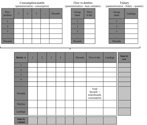
Construction de la matrice de communauté depuis un modèle Ecopath

Figure 1: Construction de la matrice de communauté depuis un modèle Ecopath

The R-code for the sensitivity analysis

The code is given for data stored in a three-sheet Excel file. The original matrix Q is stored in the “net_impacts” sheet and is obtained following steps (i) to (iv) described in Appendix C. The original matrix Q minus 20% is in the “Com_Min” sheet and the original matrix Q plus 20% in the “Com_Max” sheet. They all three give the net impact of a compartment in rows on the compartment in column.

library(RODBC)

#Specify the number of matrix Q to simulate
nb_mat <- 5000

#Connection to the Excel file and importation of the data
db <- "" #File path
channel <- odbcConnectExcel(xls.file = db)

Mini_Mat <- sqlFetch(
  channel = channel,
  ##Name of the Excel source sheet with the original matrix Q minus 20%
  sqtable = "Com_Min",
  rownames = TRUE
)
Mini_Mat <- Mini_Mat[,-1]

Maxi_Mat <- sqlFetch(
  channel = channel,
  ##Name of the Excel source sheet with the original matrix Q plus 20%
  sqtable = "Com_Max",
  rownames = TRUE
)
Maxi_Mat <- Maxi_Mat[,-1]

#Creation of two empty matrices to store the 5000 simulated Q and MTI matrices
nb_comp <- nrow(Mini_Mat)
strenght <- matrix(0,nrow=nb_comp,ncol=nb_comp*nb_mat)
strenght_adj <- matrix(0,nrow=nb_comp,ncol=nb_comp*nb_mat)

#Function to invert a matrix Q following Dambacher et al. (2002)
#With the following equation, the CM matrix must be invertible
#No compartment being only an input can be included in the model. Effect of an input may be regarded after the matrix has been inverted
#Compartment being only an output is allowed since the diagonal has been set to -1 for auto-regulation
make.adjoint2 <- function(CM,status=FALSE) {
  adj2 <- (-1)* solve(CM)*det(- (CM))
  adj2
}
#The resulting MTI matrix returns the effect of a positive perturbation in a compartment in rows on a compartment in column
#Simulation of the 5000 Q matrices by drawing q ij values from independent uniform distributions. Minimums and maximums for the distributions were defined according to Mini_Mat and Maxi_Mat

for(t in 1:nb_mat){
  col_j <- (nb_comp*t)-nb_comp
  for(i in 1:nb_comp){
    for(j in 1:nb_comp){
      strenght[i,j+col_j] <- runif(1,Mini_Mat[i,j],Maxi_Mat[i,j])
    }
  }
  #Simulation of the 5000 MTI matrices using the make.adjoint2 function to invert the 5000 Q matrices
  begin <- (nb_comp*t)-nb_comp + 1
  end <- nb_comp*t
  strenght_adj[,begin:end] <- make.adjoint2(strenght[,begin:end])
}

#Transformation of quantitative MTI values, with 1 for positive integers, 0 for nulls and -1 for negative integers
effect <- strenght_adj
for(i in 1:nb_comp){
  for(j in 1:(nb_comp*nb_mat)){
    if(strenght_adj[i,j]>0){effect[i,j] <- 1
    } else {
      if(strenght_adj[i,j]==0){effect[i,j] <- 0
      }else{
        effect[i,j] <- (-1)
      }
    }
  }
}

#Counting for each intersection the number of positive, negative and null MTI values and storage into three summary matrices ( effect_po , effect_neg and effect_nul , respectively)
effect_pos <- matrix(0,ncol = nb_comp, nrow=nb_comp)
effect_neg <- matrix(0,ncol = nb_comp, nrow=nb_comp)
effect_nul <- matrix(0,ncol = nb_comp, nrow=nb_comp)

for(t in 1:nb_mat){
  for(i in 1:nb_comp){
    for(j in 1:nb_comp){
      if(effect[i,(j+((t*nb_comp)-nb_comp))]==1){effect_pos[i,j] <- effect_pos[i,j]+1
      } else {
        if(effect[i,(j+((t*nb_comp)-nb_comp))]==(-1)){effect_neg[i,j] <- effect_neg[i,j]+1
        } else {
          effect_nul[i,j] <- effect_nul[i,j]+1
        }
      }
    }
  }
}

#For each intersection, sum of the three summary matrices should be equal to the number of simulations (here 5000). This test must return TRUE.
(sum(effect_neg + effect_pos + effect_nul - matrix(nb_mat,ncol=nb_comp,nrow=nb_comp)) == 0)

#Importation of the original Q matrix
Reference <- sqlFetch(
  channel = channel,
  #Name of the Excel source sheet with the original matrix Q
  sqtable = "net_impacts",
  rownames = TRUE
)

Reference <- as.matrix(Reference[,-1])
#Inversion of the original Q matrix resulting in the original MTI matrix
Reference <- make.adjoint2(Reference)
#Transformation of the original MTI matrix into three matrices. For a given intersection, if the original MTI value is positive (negative, null), it should be specified in the effect_pos_ref ( effect_pos_neg , effect_pos_nul ) matrix by putting the number of simulations (here 5000) at the corresponding intersection
effect_pos_ref <- matrix(0,nrow=nb_comp,ncol=nb_comp)
effect_neg_ref <- matrix(0,nrow=nb_comp,ncol=nb_comp)
effect_nul_ref <- matrix(0,nrow=nb_comp,ncol=nb_comp)

for(i in 1:nb_comp){
  for(j in 1:nb_comp){
    if(Reference[i,j] > 0){effect_pos_ref[i,j] <- nb_mat}
    if(Reference[i,j] < 0){effect_neg_ref[i,j] <- nb_mat}
    if(Reference[i,j] == 0){effect_nul_ref[i,j] <- nb_mat}
  }
}

#For each intersection, calculation of the proportion of simulations with the same sign as in the original MTI matrix
#Proportion is the final matrix used in the paper to assess sensitivity of the MTIs to 20% uncertainty in the input data.
proportion <- matrix(0,ncol = nb_comp, nrow=nb_comp)

for(i in 1:nb_comp){
  for(j in 1:nb_comp){
    if(effect_pos_ref[i,j] == nb_mat){proportion[i,j] <-(effect_pos[i,j]/nb_mat)*100}
    if(effect_neg_ref[i,j] == nb_mat){proportion[i,j] <-(effect_neg[i,j]/nb_mat)*100}
    if(effect_nul_ref[i,j] == nb_mat){proportion[i,j] <-(effect_nul[i,j]/nb_mat)*100}
  }
}