#30DayMapChallenge: 30 jours de création de cartes (3) - La Terre est une sphère

Packages

library(dplyr)
library(sf)
library(rnaturalearth)
library(tmap)
if (!requireNamespace("echarts4r", quietly = TRUE)) {
  install.packages("echarts4r")
}
if (!requireNamespace("echarts4r.assets", quietly = TRUE)) {
  remotes::install_github('JohnCoene/echarts4r.assets', upgrade = "never")
}
if (!requireNamespace("echarts4r.maps", quietly = TRUE)) {
  remotes::install_github('JohnCoene/echarts4r.maps', upgrade = "never")
}
library(echarts4r)
library(echarts4r.assets)
library(sp)
if (!requireNamespace("globe4r", quietly = TRUE)) {
 remotes::install_github("JohnCoene/globe4r", upgrade = "never")
}
library(globe4r)
library(maps)
library(ggplot2)
library(readr)
library(raster)
library(rgl)
library(geometry)

## Customize
font <- extrafont::choose_font(c("Nanum Pen", "Lato", "sans"))

my_blue <- "#1e73be"
my_theme <- function(font = "Nanum Pen", ...) {
  theme_dark() %+replace%
    theme(
      plot.title = element_text(family = font, 
                                colour = my_blue, size = 18),
      plot.subtitle = element_text(family = font, size = 15),
      # text = element_text(size = 13), #family = font, 
      plot.margin = margin(4, 4, 4, 4),
      plot.background = element_rect(fill = "#f5f5f2", color = NA),
      legend.text = element_text(family = font, size = 10),
      legend.title = element_text(family = font),
      # legend.text = element_text(size = 8),
      legend.background = element_rect(fill = "#f5f5f2"),
      ...
    )
}

Noms : Animer une sphère avec {tmap}

Trouvons des communes françaises contenant “mer/océan” dans leur nom. Notez que Maëlle Salmon a une carte similaire avec des noms de rivières et de mers dans son post de blog “French places and a sort of resolution”

# extraWD <- "." # Uncomment for the script to work
communes_L93 <- st_read(file.path(extraWD, "commune_centers.shp"))

communes_mer <- communes_L93 %>% 
  filter(grepl("\\-mer$|\\s+mer$|ocean", tolower(NOM_COM)))

# mapview::mapview(communes_mer)

# https://stackoverflow.com/questions/43207947/whole-earth-polygon-for-world-map-in-ggplot2-and-sf/43278961#43278961
crs <- "+proj=laea +lat_0=52 +lon_0=10 +x_0=4321000 +y_0=3210000 +datum=WGS84 +units=m +no_defs"

world_ne <- ne_countries(scale = 50, type = "countries", returnclass = "sf") %>%
  select(iso_a3, iso_n3, admin, continent)

sphere <- st_graticule(ndiscr = 10000, margin = 10e-6) %>%
  st_transform(crs = crs) %>%
  st_convex_hull() %>%
  summarise(geometry = st_union(geometry))

show_dist <- function(dist, name) {
  
  # Crop World to area around France
  france_large <- world_ne %>% 
    st_crop(communes_mer %>% 
              st_buffer(dist = units::set_units(dist, "km")) %>% 
              st_transform(crs = st_crs(world_ne))) %>% 
        st_transform(crs)
  
  # Plot
  tm <- tm_shape(sphere) +
    tm_fill(col = "#D8F4FF") +
   tm_graticules() +
   tm_shape(france_large, is.master = TRUE) +
    tm_polygons() +
   tm_shape(communes_mer) +
    tm_symbols(col = my_blue) +
   tm_layout() +
    tm_credits("{sf} - {tmap} - @statnmap",
             position = c(0.38, -0.01),
             size = 1.3, fontfamily = "Nanum Pen",
             col = "grey90") +
  tm_layout(
    main.title = "Cities with 'mer' or 'ocean' in names",
    main.title.color = my_blue,
    main.title.fontfamily = "Nanum Pen",
    main.title.size = 1.75,
    title = "Why are there 2 cities named 'mer' in the mainland?",
    title.fontfamily = "Nanum Pen",
    title.bg.color = "white",
    title.bg.alpha = 0.7,
    # Margin to allow legend
    inner.margins = 0,
    # Colours
    outer.bg.color = c("#E6EFFA")#,
    # bg.color = my_blue #"grey60"
  )
  
  tmap_save(tm, filename = file.path(extraWD, "gif", paste0(name, ".jpg")),
          width = 1024, height = 512, units = "px",
          dpi = 100)
}

if (!dir.exists(file.path(extraWD, "gif"))) {
  dir.create(file.path(extraWD, "gif"))
}

seq_dist <- seq(1, 10000, by = 500)
seq_names <- formatC(seq_along(seq_dist), width = 3, flag = 0)
purrr::walk2(seq_dist, seq_names, ~show_dist(.x, .y))

# Create gif
img_frames <- list.files(file.path(extraWD, "gif"),
                         full.names = TRUE)

magick::image_write_gif(magick::image_read(img_frames), 
                          path = file.path(extraWD, "names.gif"), 
                          delay = 3/length(img_frames))

Lieux : Créer un globe terrestre HTML interactif avec {echarts4r}

Cartographions les 7 merveilles du monde antique : Grande Pyramide de Guizeh, Jardins suspendus de Babylone, Temple d’Artémis, Statue de Zeus à Olympie, Mausolée à Halicarnasse, Colosse de Rhodes et Phare d’Alexandrie.
J’ai récupéré les coordonnées sur la page de Wikipédia “Sept Merveilles du Monde Antique”, où toutes n’ont pas le même format. Pour certaines coordonnées, j’utilise char2dms() du package {sp}.
Pour cette cartes, j’utilise le package {echarts4r} de John Coene pour la première fois. Je m’inspire de l’article de blog de Jesus M. Castagnetto (@jmcastagnetto) “Chart, map and globe showing nuclear explosions (1945-1998)” avec le code du dépôt Github correspondant.
J’ai choisi de rendre le résultat sous forme de gif au lieu du widget html interactif de {echarts4r}. J’ai utilisé {htmlwidgets}, {pagedown} et {magick} pour créer le gif de la page HTML.

# 7 Wonders geographic positions
wonders_wgs84 <- tribble(
  ~id, ~name, ~lat, ~long,
  1, "Giza", as.numeric(char2dms("29d58'45.03\"N")), as.numeric(char2dms("31d08'03.69\"E")),
  2, "Babylon", 32.5355, 44.4275,
  3, "Ephesus", as.numeric(char2dms("37d56'59\"N")), as.numeric(char2dms("27d21'50\"E")),
  4, "Olympia", as.numeric(char2dms("37d38'16.3\"N")), as.numeric(char2dms("21d37'48\"E")),
  5, "Halicarnassus", 37.0379, 27.4241,
  6, "Rhodes", as.numeric(char2dms("36d27'04\"N")), as.numeric(char2dms("28d13'40\"E")),
  7, "Alexandria", as.numeric(char2dms("31d12'50\"N")), as.numeric(char2dms("29d53'08\"E"))
) %>% 
  st_as_sf(coords = c("long", "lat"), crs = 4326, remove = FALSE)

e <- wonders_wgs84 %>% 
  # x-axis (longitude for maps)
  e_charts(long) %>% 
  # globe
  e_globe(
    environment = ea_asset("starfield"),
    base_texture = ea_asset("world topo"),
    height_texture = ea_asset("world topo"),
    globeOuterRadius = 100
  ) %>% 
  # create points, with y-axis column
  e_scatter_3d(lat, id, coord_system = "globe", blendMode = 'lighter') %>% 
  e_visual_map(min = 1, max = 7,
               inRange = list(symbolSize = c(8, 10))) %>% 
  e_toolbox_feature(
    feature = c("saveAsImage", "restore")
  ) %>%
  e_title(
    "Seven Wonders of the Ancient World",
    "Source: @statnmap"
  )


# save as html
htmlwidgets::saveWidget(e, file = file.path(extraWD, "echarts4r-places.html"))

# Create some snapshots of the html
dir_gif <- file.path(extraWD, "gif-globe")
if (!dir.exists(dir_gif)) {dir.create(dir_gif)}
wait_time <- seq(0, 35, by = 2)
for (i in 10:length(wait_time)) {
  pagedown::chrome_print(
    input = file.path(extraWD, "echarts4r-places.html"),
    output = file.path(
      dir_gif,
      paste0("echarts4r-places-", 
             formatC(i, flag = 0, width = 3),
             ".jpeg")
    ),
    format = "jpeg",
    wait = wait_time[i],
    timeout = wait_time[i] + 20)
}

# Create gif
img_frames <- list.files(dir_gif, full.names = TRUE)

magick::image_write_gif(magick::image_read(img_frames), 
                          path = file.path(extraWD, "places.gif"), 
                          delay = 3/length(img_frames))

Zones : Diviser des zones selon une sphère avec {sf}

J’ai eu habité en Loire-atlantique comme vous l’aurez peut-être compris si vous avez lu le premier article de ce défi cartographique. Ce département est divisé en deux parties par la Loire, et nous avons l’habitude de nommer ces deux parties: “Nord Loire” et “Sud Loire”. C’est aussi, à mon avis, la limite que je mettrais pour diviser la France entre le Nord et le Sud. Voyons voir où cela coupe le monde….

• Récupérer la carte hydrographique de la France sur le site de l’IGN
• Récupérer les rivières du monde avec {mapdata}
• Trouver la latitude de cette ligne en utilisant {mapview} : environ 47,28° si je me réfère à l’estuaire de la Loire
• Créer une fine couche polygone autour du Monde, définie par cette latitude
• Diviser le département en deux parties
• Diviser la France en deux parties
• Diviser le monde en deux parties
• Créer la carte avec {ggplot2}

# France
France_l93 <- st_read(file.path(extraWD, "DEPARTEMENT.shp"))
France_wgs84 <- France_l93 %>% 
  st_transform(crs = 4326)

# Loire river from IGN
Loire_l93 <- st_read(file.path(extraWD, "Loire.shp"))
Loire_wgs84 <- Loire_l93 %>% 
  st_transform(crs = 4326)

# {mapdata} World rivers
rivers_wgs84 <- map('rivers', plot = FALSE) %>% 
  maptools::map2SpatialLines() %>% 
  st_as_sf() %>% 
  st_set_crs(4326) %>% 
  mutate(id = 1:n())

# LA cut ----
# Cut Loire atlantique with river
Loire_buf_l93 <- Loire_l93 %>% 
  st_buffer(dist = units::set_units(1500, "m"))

LA_cut_l93 <- France_l93 %>% 
  filter(CODE_DEPT == 44) %>%  
  st_difference(Loire_buf_l93) %>% 
  st_cast("POLYGON") %>% 
  mutate(id = 1:n())

# mapview::mapview(France_44_inter)
g1 <- ggplot() +
  geom_sf(data = LA_cut_l93, aes(fill = as.character(id))) +
  guides(fill = FALSE) +
  theme(axis.text = element_blank(),
        axis.ticks = element_blank())

# France cut ----
# Find limit
# mapview::mapview(rivers_wgs84)
lat_limit <- 47.28

# Create line to separate North-South
north_line_fr <- matrix(
  c(-5, lat_limit, 
    10, lat_limit),
  ncol = 2, byrow = TRUE
)
line_north_fr_wgs84 <- st_linestring(north_line_fr) %>% 
  st_sample(50) %>% 
  st_cast("LINESTRING") %>% 
  st_sfc(crs = 4326) 

line_north_fr_buf_wgs84 <- line_north_fr_wgs84 %>% 
  st_buffer(dist = 0.01)
  # st_buffer(dist = units::set_units(1500, "m"))

# Cut France in 2 parts
Fr_cut_wgs84 <- France_wgs84 %>% 
  st_union() %>% 
  st_difference(line_north_fr_buf_wgs84) %>% 
  st_cast("POLYGON") %>% 
  st_sf() %>% 
  mutate(id = sample(1:n()))

g2 <- ggplot() +
  geom_sf(data = Fr_cut_wgs84, aes(fill = as.character(id))) +
  geom_sf(data = line_north_fr_buf_wgs84, fill = "red") +
  coord_sf(crs = 2154) +
  guides(fill = FALSE) +
  theme(axis.text = element_blank(),
        axis.ticks = element_blank())

# World cut ----
crs <- "+proj=laea +lat_0=52 +lon_0=10 +x_0=4321000 +y_0=3210000 +datum=WGS84 +units=m +no_defs"

# Get World
world_ne <- rnaturalearth::ne_countries(returnclass = "sf")

# Create line to separate North-South
north_line <- matrix(
  c(-180, lat_limit, 
    180, lat_limit),
  ncol = 2, byrow = TRUE
)
line_north_wgs84 <- st_linestring(north_line) %>% 
  st_sample(300) %>% 
  st_cast("LINESTRING") %>% 
  st_sfc(crs = 4326) 
line_north_buf_wgs84 <- line_north_wgs84 %>% 
  st_buffer(dist = 0.01)

# Cut World in 2 parts
World_cut_wgs84 <- world_ne %>% 
  st_union() %>% 
  st_difference(line_north_buf_wgs84) %>% 
  st_cast("POLYGON") %>% 
  st_sf() %>% 
  mutate(id = sample(1:n()))

g3 <- ggplot() +
  geom_sf(data = World_cut_wgs84, aes(fill = as.character(id))) +
  geom_sf(data = line_north_buf_wgs84, colour = "red") +
  coord_sf(crs = crs) +
  guides(fill = FALSE)


p <- cowplot::plot_grid(
  g1, g2, g3, nrow = 1,
  labels = "What is North really?", 
  label_fontfamily = "Nanum Pen",
  label_colour = my_blue, label_size = 50)

jpeg(filename = file.path(extraWD, "zones.jpg"),
     width = 1024, height = 512, units = "px", pointsize = 12,
     quality = 75
)
p
dev.off()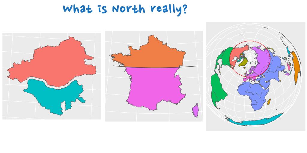

Globe: Créer un globe interactif avec {globe4r}

Y a-t-il une meilleure façon de créer un globe que d’utiliser “globe.js” ? Jouons rapidement avec le package {globe4r} John Coene.
Mon ordinateur a un peu trop souffert avec cette carte interactive. J’ai donc pris une capture d’écran pour éviter de faire souffrir votre ordinateur à l’ouverture de cet article. On dit merci qui ?

# France
France_l93 <- st_read(file.path(extraWD, "DEPARTEMENT.shp"))
France_wgs84 <- France_l93 %>% 
  st_transform(crs = 4326)

# Create globe
create_globe() %>% 
globe_choropleth(
  data = France_wgs84,
  coords(
    polygon = CODE_REG,
    cap_color = CODE_REG
  ))

# convert to JSON
india_geojson <- geojsonio::geojson_list(France_wgs84)

regions <- india_geojson$features %>% 
  purrr::map("properties") %>% 
  purrr::map("CODE_REG") %>% 
  unlist()

mock_data <- data.frame(
  CODE_REG = regions,
  value = as.numeric(as.character(regions))
)

globe <- create_globe() %>% 
  globe_choropleth(
    data = mock_data,
    coords(
      polygon = CODE_REG,
      cap_color = value,
      altitude = value
    ),
    polygons = india_geojson
  ) %>% 
  globe_pov(47, 2, 0.75) %>% 
  scale_choropleth_cap_color(
    palette = scales::viridis_pal()(5)) %>% 
  scale_choropleth_altitude(max = 0.1) %>%
  show_graticules()
 
# save as html
htmlwidgets::saveWidget(globe, file = file.path(extraWD, "globe4r-globe.html"))

# Print a snapshot - To long to render
# pagedown::chrome_print(
#   input = file.path(extraWD, "globe4r-globe.html"),
#   output = file.path(extraWD,"globe4r-globe.jpeg"),
#   format = "jpeg",
#   wait = 10,
#   timeout = 60)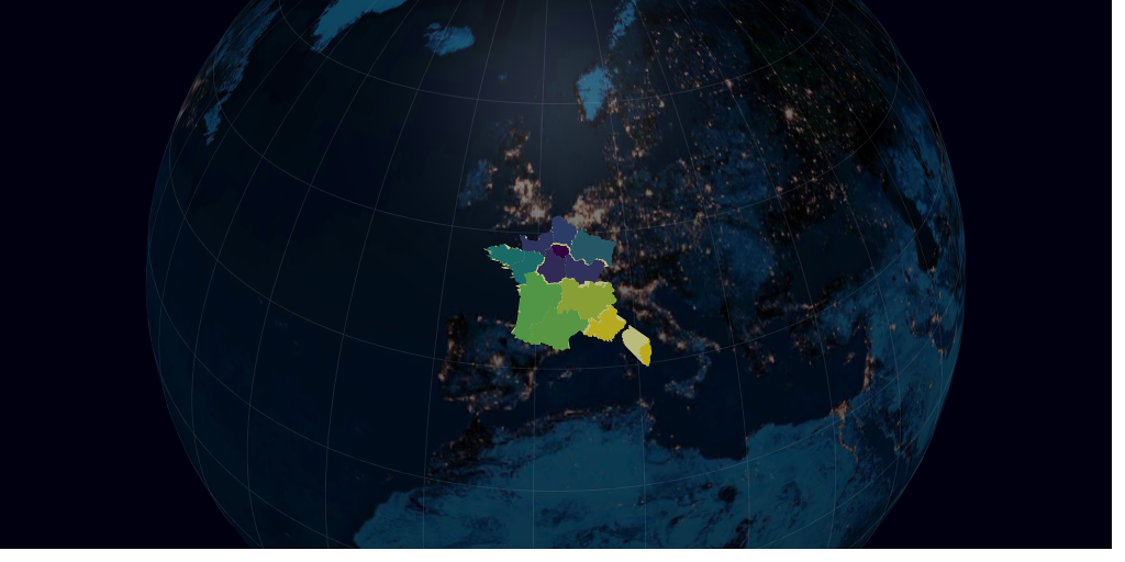

Urbain·e : Créer une vue du globe et un encart avec {ggplot2}

Au cours de ce défi, j’ai montré quelques cartes comme la distribution des bars en France qui est susceptible d’être corrélée avec la distribution de la population. Aujourd’hui, il est temps de montrer directement cette carte de la population française.
Dans le jeu de données world.cities de {maps}, seules les villes de plus de 40000 habitants sont représentées, ainsi que toutes les capitales de toute taille de population (et quelques autres petites villes). A quoi ressemble la France si on sépare les villes avec cette limite de 40000 habitants ?

# France data
communes_L93 <- st_read(file.path(extraWD, "commune_centers.shp"))
communes_big_L93 <- communes_L93 %>% 
  mutate(big = if_else(POPULATION >= 40000, TRUE, FALSE))

# World crs ----
crs <- "+proj=laea +lat_0=52 +lon_0=10 +x_0=4321000 +y_0=3210000 +datum=WGS84 +units=m +no_defs"

g1 <- ggplot() + 
  geom_sf(data = communes_big_L93,
          aes(colour = big, size = POPULATION), 
              show.legend = "point") +
  # scale_size_continuous(trans = "log10") +
  scale_size(range = c(0, 4)) +
  scale_colour_viridis_d(name = "Big cities?") +
    labs(
    title = "French cities population",
    subtitle = "Where are big cities (>=40000 inh.)?",
    caption = "ggplot2 - @statnmap - source: ign.fr",
    x = NULL, y = NULL,
    fill = "Number"
  ) +
  coord_sf(crs = 2154) +
  my_theme()

ggsave(plot = g, filename = file.path(extraWD, "urban.jpg"),
       width = 20, height = 10, units = "cm",
       dpi = 200)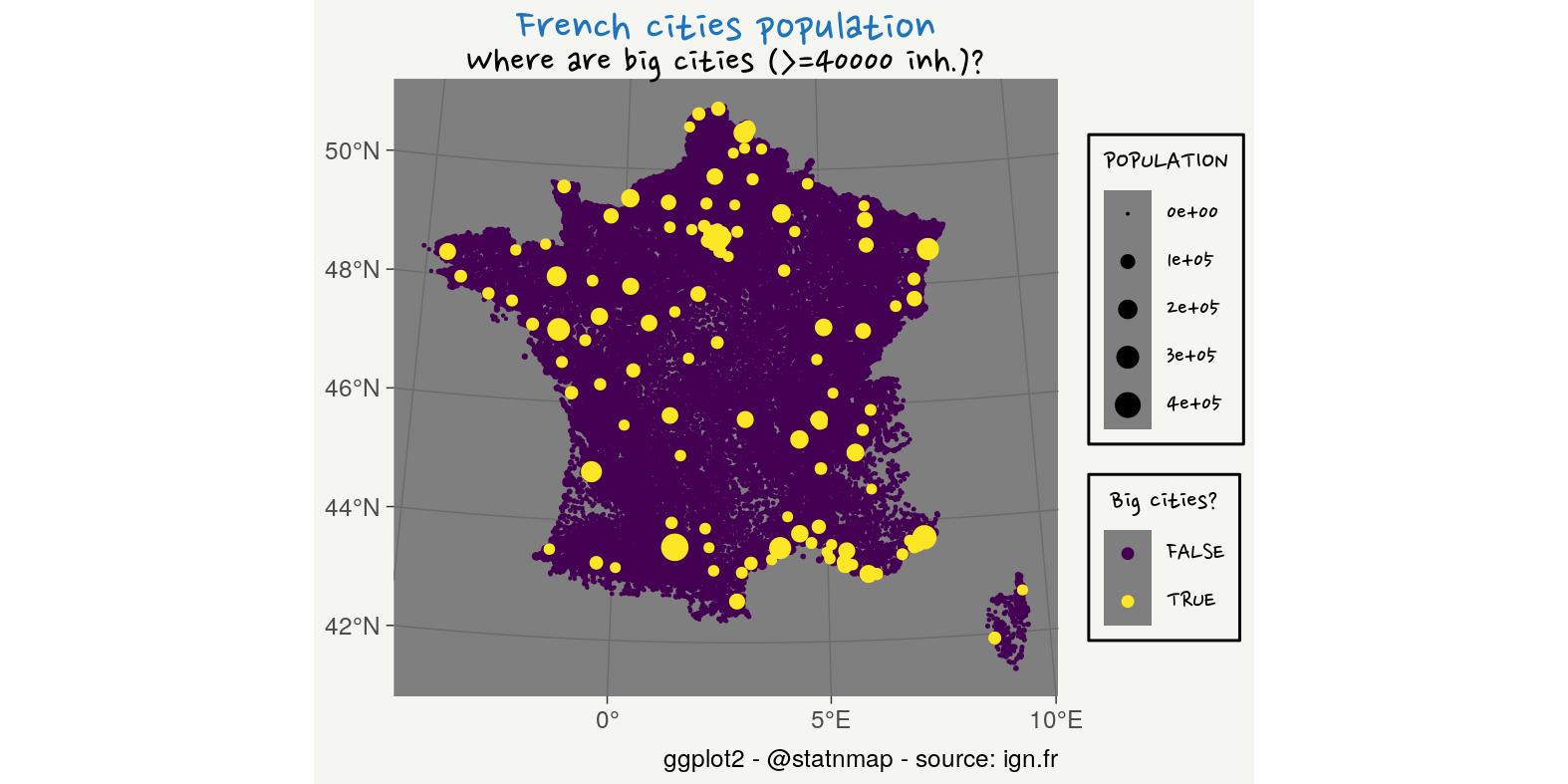

Voyons un peu la situation de la France à l’échelle du monde.

# World data
data(world.cities)

w_cities <- world.cities %>% 
  st_as_sf(coords = c("long", "lat"), crs = 4326) %>% 
  rename(POPULATION = pop) %>% 
  mutate(big = if_else(POPULATION >= 40000, TRUE, FALSE))

# Ocean as blue
graticule <- st_graticule(ndiscr = 10000, margin = 10e-6) %>%
  st_transform(crs = crs) 

sphere <- st_graticule(ndiscr = 10000, margin = 10e-6) %>%
  st_transform(crs = crs) %>%
  st_convex_hull() %>%
  summarise(geometry = st_union(geometry))

# France inset
g1 <- ggplot() + 
  geom_sf(data = communes_big_L93,
          aes(colour = big, size = POPULATION), 
              show.legend = "point") +
  # scale_size_continuous(trans = "log10") +
  scale_size(range = c(0, 2)) +
  scale_colour_viridis_d(name = "Big cities?") +
  guides(size = FALSE, colour = FALSE) +
  labs(x = NULL, y = NULL) +
  theme(
    axis.title = element_blank(),
    axis.text = element_blank(),
    axis.ticks = element_blank(),
    panel.background = element_rect(fill = my_blue),
    plot.margin = margin(0,0,0,0)
  )

# World
g2 <- ggplot() + 
  geom_sf(data = sphere, fill = my_blue) +
  geom_sf(data = graticule, size = 0.1) +
  geom_sf(data = w_cities, aes(colour = big, size = POPULATION), 
              show.legend = "point") +
  geom_sf(data = communes_big_L93,
          aes(colour = big, size = POPULATION), 
              show.legend = "point") +
  # scale_size_continuous(trans = "log10") +
  scale_size(range = c(0, 2)) +
  scale_colour_viridis_d(name = "Big cities?") +
    labs(
    title = "World cities population",
    subtitle = "Where are big cities (>=40000 inh.)?",
    caption = "ggplot2 - @statnmap - source: ign.fr",
    x = NULL, y = NULL,
    fill = "Number"
  ) +
  coord_sf(crs = crs) +
  my_theme() +
  # 
  # ggplot() +
  # geom_sf(data = sphere, fill = my_blue) +
  # coord_sf(crs = crs) +
  annotation_custom(
    grob = ggplotGrob(g1),
    xmin = 9e6, xmax = Inf, ymin = -Inf, ymax = 0)

ggsave(plot = g2, filename = file.path(extraWD, "urban_world.jpg"),
       width = 20, height = 10, units = "cm",
       dpi = 200)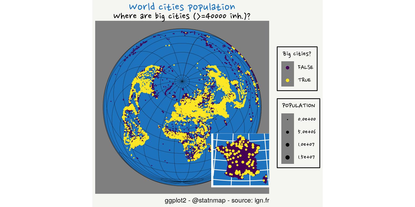

Rural : Créer un zoom animé du globe avec {tmap}

J’ai trouvé un jeu de données des villes françaises où il existe une Appellation d’Origine Protégée ou Contrôlée et une liste sur un PDF de tous les fromages AOP/AOC sur le site de l’INAO

• Nettoyer les jeux de données avec {thinkr}.
• Fusionner avec la table des noms de fromages
• Fusionner avec la carte des centres des villes
  • La fusion n’est pas parfaite car certains ID de villes (INSEE_COM) ne sont pas toutes identiques dans les deux bases. J’ai donc terminé avec une fusion sur le nom. Certaines villes manquent encore de coordonnées.

# Cities centers
communes_L93 <- st_read(file.path(extraWD, "commune_centers.shp"))

# Cities with AOP
data_aop <- read_csv2(file.path(extraWD, "2019-11-05-comagri-communes-aires-ao.csv"), locale = locale(encoding = "latin1")) %>% 
  mutate(AOP = thinkr::clean_vec(`Aire géographique`, unique = FALSE))

# AOP for Cheese
names_cheese <- read_csv(file.path(extraWD, "Fromages_fr.csv")) %>% 
  mutate(AOP = thinkr::clean_vec(Fromages, unique = FALSE))

# Filter only cheese names
data_ao_cheese <- data_aop %>% 
  inner_join(names_cheese)

data_ao_cheese_L93 <- communes_L93 %>% 
  right_join(data_ao_cheese, by = c("INSEE_COM" = "CI"))

# Remove empty
data_ao_cheese_insee_L93 <- data_ao_cheese_L93 %>% 
  filter(!st_is_empty(.))

# Get empty and merge with name
data_ao_cheese_empty <- data_ao_cheese %>% 
  anti_join(data_ao_cheese_insee_L93, by = c("CI" = "INSEE_COM")) %>% 
  mutate(COM = toupper(Commune)) 

data_ao_cheese_name_L93 <- communes_L93 %>% 
  right_join(data_ao_cheese_empty, by = c("NOM_COM" = "COM")) %>% 
  filter(!st_is_empty(.)) %>% 
  select(-CI)

# Merge insee + name
data_ao_cheese_complete_l93 <- data_ao_cheese_insee_L93 %>% 
  rbind(data_ao_cheese_name_L93)

# Some still do not have coords  

tm_shape(data_ao_cheese_complete_l93) +
  tm_symbols(col = my_blue, size = 0.1, shape = 20)

# Map
crs <- "+proj=laea +lat_0=52 +lon_0=10 +x_0=4321000 +y_0=3210000 +datum=WGS84 +units=m +no_defs"

# Transformation requires st_make_valid()
world_ne <- ne_countries(scale = 50, type = "countries", returnclass = "sf") %>%
  select(iso_a3, iso_n3, admin, continent) %>% 
  st_transform(crs = crs) %>%
  lwgeom::st_make_valid() 

# Background
graticule <- st_graticule(ndiscr = 10000, margin = 10e-6) %>%
  st_transform(crs = crs)
sphere <- graticule %>%
  st_convex_hull() %>%
  summarise(geometry = st_union(geometry))

# Function
show_dist <- function(
  world_ne,
  dist, name, points, 
  crs = "+proj=laea +lat_0=52 +lon_0=10 +x_0=4321000 +y_0=3210000 +datum=WGS84 +units=m +no_defs") {
  
  points <- st_transform(points, crs)
  
  # Get bbox buffer
  bbox_pt_buffer <- points %>% 
    st_bbox() %>%
    st_as_sfc() %>% 
    st_transform(crs = st_crs(world_ne)) %>% 
    st_buffer(dist = units::set_units(dist, "km"))
  
  # Crop World to area around France
  france_large <- world_ne %>% 
    st_crop(bbox_pt_buffer) %>% 
    st_transform(crs)

  # Plot
  tm <- tm_shape(sphere) +
    tm_fill(col = "#D8F4FF") +
   # tm_graticules() +
    tm_shape(graticule) +
    tm_lines(col = "grey30", lwd = 0.5) +
   tm_shape(france_large, is.master = TRUE) +
    tm_polygons() +
   tm_shape(points) +
    tm_symbols(col = my_blue, size = 0.1, shape = 20) +
   tm_layout() +
    tm_credits("{sf} - {tmap} - @statnmap",
             position = c(0.38, -0.01),
             size = 1.3, fontfamily = "Nanum Pen",
             col = "grey90") +
  tm_layout(
    main.title = "French cities where there is AOP cheese",
    main.title.color = my_blue,
    main.title.fontfamily = "Nanum Pen",
    main.title.size = 1.75,
    title = "What would be France without cheese?",
    title.fontfamily = "Nanum Pen",
    title.bg.color = "white",
    title.bg.alpha = 0.7,
    # Margin to allow legend
    inner.margins = 0,
    outer.margins = c(0.01, 0.17, 0.01, 0.17),
    # Colours
    outer.bg.color = c("#E6EFFA")#,
    # bg.color = my_blue #"grey60"
  )
  
  tmap_save(tm, filename = file.path(extraWD, "gif-rural", paste0(name, ".jpg")),
          width = 1024, height = 512, units = "px",
          dpi = 100)
}

# Create each frame
# show_dist(world_ne = world_ne,
#           dist = 500,
#           name = "001",
#           points = data_ao_cheese_complete_l93)

if (!dir.exists(file.path(extraWD, "gif-rural"))) {
  dir.create(file.path(extraWD, "gif-rural"))
}

seq_dist <- seq(1, 15000, by = 500)
seq_names <- formatC(seq_along(seq_dist), width = 3, flag = 0)
purrr::walk2(
  seq_dist, seq_names,
  ~show_dist(dist = .x,
             name = .y,
             world_ne = world_ne,
             points = data_ao_cheese_complete_l93))

# Create gif
img_frames <- list.files(
  file.path(extraWD, "gif-rural"),
  full.names = TRUE)

magick::image_write_gif(
  magick::image_read(img_frames), 
  path = file.path(extraWD, "rural.gif"), 
  delay = 3/length(img_frames))

Environnement : Dessiner un raster sur une sphère avec {rgl}

Nous téléchargeons les données de Worldclim avec la fonction getData du package {raster}. Dans cette carte, je vais montrer une variable d’environnement : Les précipitations annuelles (BIO12).

• Télécharger le jeu de données
• Réduire la résolution
• Tracé sur une sphère 3D suivant mon article de blog Interpolation spatiale sur le globe terrestre 3D en utilisant {GeoDist}, Constrained distance calculation and associated geotools et {rgl}

prec <- raster::getData("worldclim", var = "bio", 
                path = extraWD, res  = 10)

bio12 <- raster(prec, 12) %>% 
  raster::aggregate(fact = 5, fun = sum)
# plot(bio12)

# Transform as cartesian coordinates
r.cart <- data.frame(GeoDist::sph2car(coordinates(bio12)))
# Triangulate entire globe directly with geometry ----
tri3d <- geometry::convhulln(r.cart)
r.cart.tri <- r.cart[t(tri3d), ] %>%
  mutate(n = c(t(tri3d)))

# Define a vector of colors for predictions
n.break <- 20
colors <- alpha(colorRampPalette(c("#ffffcc", my_blue))(n.break), .4)
brk <- seq(minValue(bio12), maxValue(bio12), len = n.break + 1)
pred.col <- colors[as.numeric(as.character(values(
  raster::cut(bio12, breaks = brk, include.lowest = TRUE))))]

# Print in 3d
triangles3d(r.cart.tri$x,
            r.cart.tri$y,
            r.cart.tri$z,
            col = pred.col[r.cart.tri$n],
            alpha = 0.9,
            specular = "black")
# Black background
rgl.bg(color = c("black"))
# Add Earth rotation axe
segments3d(x = c(0,0),
           y = c(0,0),
           z = c(min(r.cart.tri$z)*1.2, 
                 max(r.cart.tri$z)*1.2),
           col = "white",
           lwd = 2)

# Map world on the 3d sphere ----
library(rworldmap)
data(countriesCoarse)

for (i in 1:nrow(countriesCoarse)) { # i <- 1
  Pols <- countriesCoarse@polygons[[i]]  
  for (j in 1:length(Pols)) { # j <- 1
    lines3d(data.frame(GeoDist::sph2car(
      countriesCoarse@polygons[[i]]@Polygons[[j]]@coords
    )), col = "white", lwd = 2)
  }
}

# Rotate and save as gif
# extraWD: directory where to save img of rotation
nb.img <- 45
angle.rad <- seq(0, 2*pi, length.out = nb.img)
# NorthPole on top, Europe-Africa in front.
uM0 <- rotationMatrix(-pi/2, 1, 0, 0) %>%
  transform3d(rotationMatrix(-2, 0, 0, 1)) %>%
  transform3d(rotationMatrix(-pi/12, 1, 0, 0))
# Change viewpoint
rgl.viewpoint(theta = 0, phi = 0, fov = 0, zoom = 0.7,
              userMatrix = uM0)

if (!dir.exists(file.path(extraWD, "gif-envt"))) {
  dir.create(file.path(extraWD, "gif-envt"))
}
for (i in 1:nb.img) {
  # Calculate matrix rotation
  uMi <- transform3d(uM0, rotationMatrix(-angle.rad[i], 0, 0, 1))
  # Change viewpoint
  rgl.viewpoint(theta = 0, phi = 0, fov = 0, zoom = 0.7,
                userMatrix = uMi)
  # Save image
  filename <- file.path(extraWD, "gif-envt", paste0(formatC(i, digits = 1, flag = "0"), ".png"))
  rgl.snapshot(filename)    
}
# Create gif
# Create gif
img_frames <- list.files(
  file.path(extraWD, "gif-envt"),
  full.names = TRUE)

magick::image_write_gif(
  magick::image_read(img_frames), 
  path = file.path(extraWD, "envt.gif"), 
  delay = 3/length(img_frames))

Maintenant que vous avez vu différentes possibilités de créer des cartes avec une vue du globe terrestre avec R, vous pouvez lire les articles des autres semaines du défi :

• Créer des cartes dans R avec {ggplot2}
• Créer des cartes dans R avec {tmap}

Comme toujours, le code et les données sont disponibles sur https://github.com/statnmap/blog_tips

# Biblio with {chameleon}
tmp_biblio <- tempdir()
attachment::att_from_rmd("2019-11-22-30daymapchallenge-building-maps-3-earth-is-sphere.Rmd", inside_rmd = TRUE) %>% 
  chameleon::create_biblio_file(
    out.dir = tmp_biblio, to = "html", edit = FALSE,
    output = "packages")
htmltools::includeMarkdown(file.path(tmp_biblio, "bibliography.html"))

@misc{Roche2019#30Da,
    author = {Rochette Sébastien},
    title = {#30DayMapChallenge: 30 jours de création de cartes (3) - La Terre est une sphère},
    url = {https://statnmap.com/fr/2019-11-22-30daymapchallenge-creer-cartes-3-la-terre-est-une-sphere/},
    year = {2019}
  }