#30DayMapChallenge: 30 jours de création de cartes (1) - ggplot2

posté le 8 nov. 2019 · 2359 mots. · 12 minutes de lecture.

spatial · r-scripts · geohacking

rstatsFR · raster · sf · ggplot2

Le défi #30DayMapChallenge a été lancé par Topi Tjukanov sur Twitter. Il est ouvert à tous ceux qui souhaitent créer une carte, quelque soit le logiciel. Dans ce post de blog, je vais montrer des cartes réalisée avec R. Je m’ajoute aussi des contraintes à moi-même pour le plaisir. Cette semaine, j’utiliserai {ggplot2} pour créer mes cartes.

Packages

library(dplyr)
library(sf)
library(raster)
library(ggplot2)
library(readr)
library(tmap)
# library(hexbin)

## Customize
# Test for font family
# extrafont::font_import(prompt = FALSE)
font <- extrafont::choose_font(c("Nanum Pen", "Lato", "sans"))

my_blue <- "#1e73be"
my_theme <- function(font = "Nanum Pen", ...) {
  theme_dark() %+replace%
    theme(
      plot.title = element_text(family = font, 
                                colour = my_blue, size = 18),
      plot.subtitle = element_text(family = font, size = 15),
      # text = element_text(size = 13), #family = font, 
      plot.margin = margin(4, 4, 4, 4),
      plot.background = element_rect(fill = "#f5f5f2", color = NA),
      legend.text = element_text(family = font, size = 10),
      legend.title = element_text(family = font),
      # legend.text = element_text(size = 8),
      legend.background = element_rect(fill = "#f5f5f2"),
      ...
    )
}

Données

La Loire-atlantique en France

# extraWD <- "." # Uncomment for the script to work
# Read shapefile "Departement.shp"
France_L93 <- st_read(file.path(extraWD, "DEPARTEMENT.shp"), quiet = TRUE)
LoireATl_L93 <- st_read(file.path(extraWD, "Intersect_ZE_L93.shp"), quiet = TRUE)

# Create polygon for oceanic area (difference with terrestrial)
LoireATl_ocean_L93 <- st_bbox(LoireATl_L93) %>%
  st_as_sfc()  %>% 
  st_difference(st_union(LoireATl_L93))

ggplot(LoireATl_ocean_L93) +
  geom_sf(fill = my_blue) +
  labs(
    title = "bbox difference with terrestrial"
  ) +
  theme_dark()

# Read trafic in Loire-atlantique 2010, 2013
trafic_L93 <- st_read(file.path(extraWD, "trafic_L93.shp"), quiet = TRUE)

# Trafic merged with roads
RoadsMergeTrafic_Dpt44_L93 <- st_read( 
  file.path(extraWD, "RoadsMergeTrafic_Dpt44_L93.shp"),
  quiet = TRUE) %>% 
  st_line_merge()

Points : Positions géographiques et multi-graphiques avec {ggplot2}

ggplot() + 
  geom_sf(data = LoireATl_ocean_L93, colour = NA, fill = my_blue, alpha = 0.75) +
  geom_sf(data = LoireATl_L93, colour = "grey80", fill = NA) +
  geom_sf(data = trafic_L93, aes(size = TV), 
          colour = "white", alpha = 0.5, 
          inherit.aes = FALSE, show.legend = "point") +
  facet_wrap(~ANNEE_REF) +
  coord_sf(crs = st_crs(trafic_L93),
           xlim = c(st_bbox(trafic_L93)$xmin, st_bbox(trafic_L93)$xmax),
           ylim = c(st_bbox(trafic_L93)$ymin, st_bbox(trafic_L93)$ymax)) +
  scale_colour_gradientn(
    "Nombre",
    colours = RColorBrewer::brewer.pal(9, "YlOrRd"),
    trans = "log",
    breaks = c(400, 1000, 3000, 8000, 22000)
    ) +
  scale_size(range = c(0.25, 4)) +
  # guides(size = FALSE) +
  labs(x = "", y = "", 
       title = "Trafic sur les routes de Loire-atlantique",
       subtitle = "Nombre de voitures (moyenne journalière au point de contrôle)",
       caption = "@statnmap; Source: data.loire-atlantique.fr",
       size = "Nombre\nvéhicules") +
  theme_dark(base_size = 10) +
  theme(plot.title = element_text(colour = my_blue))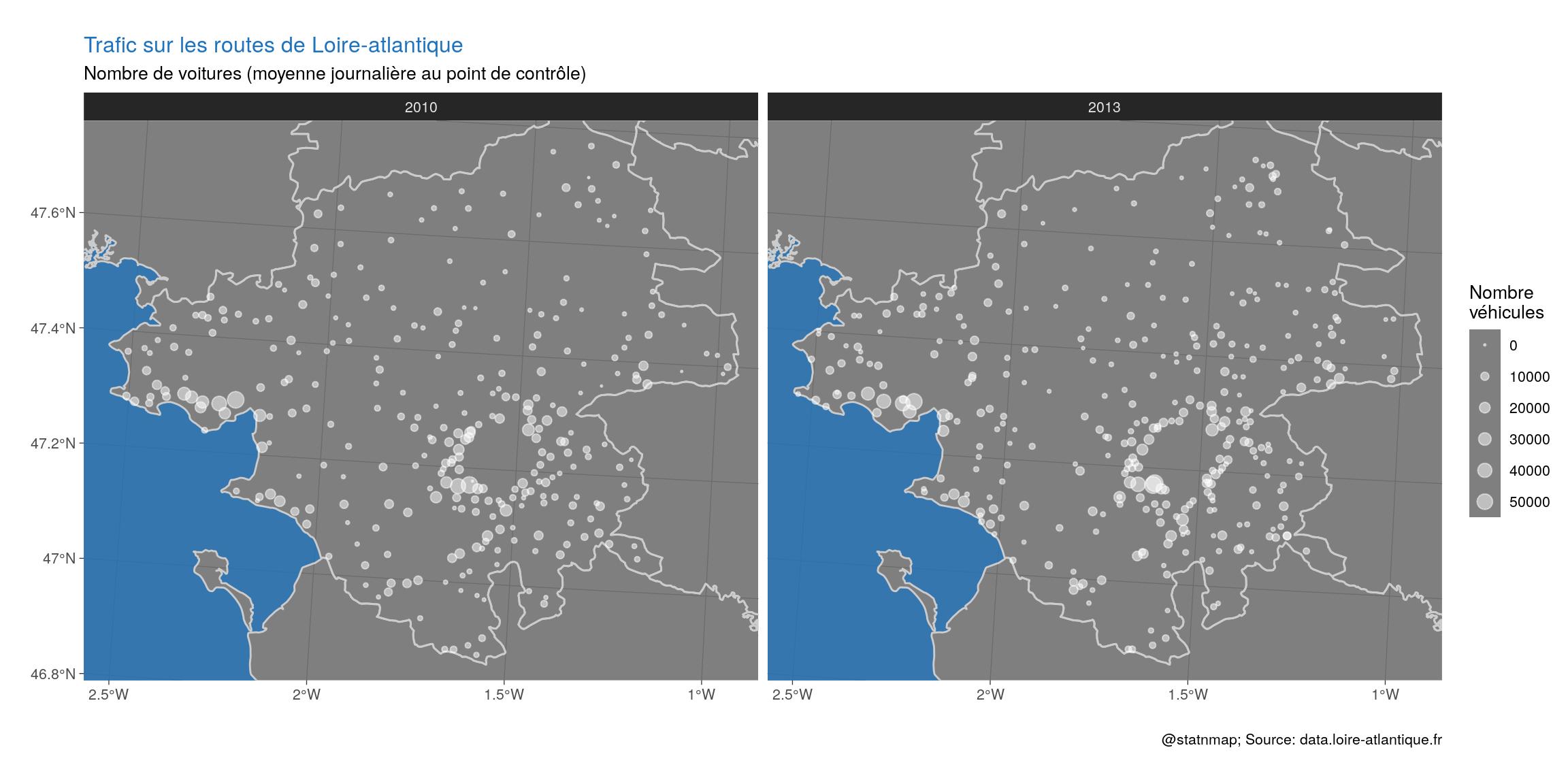

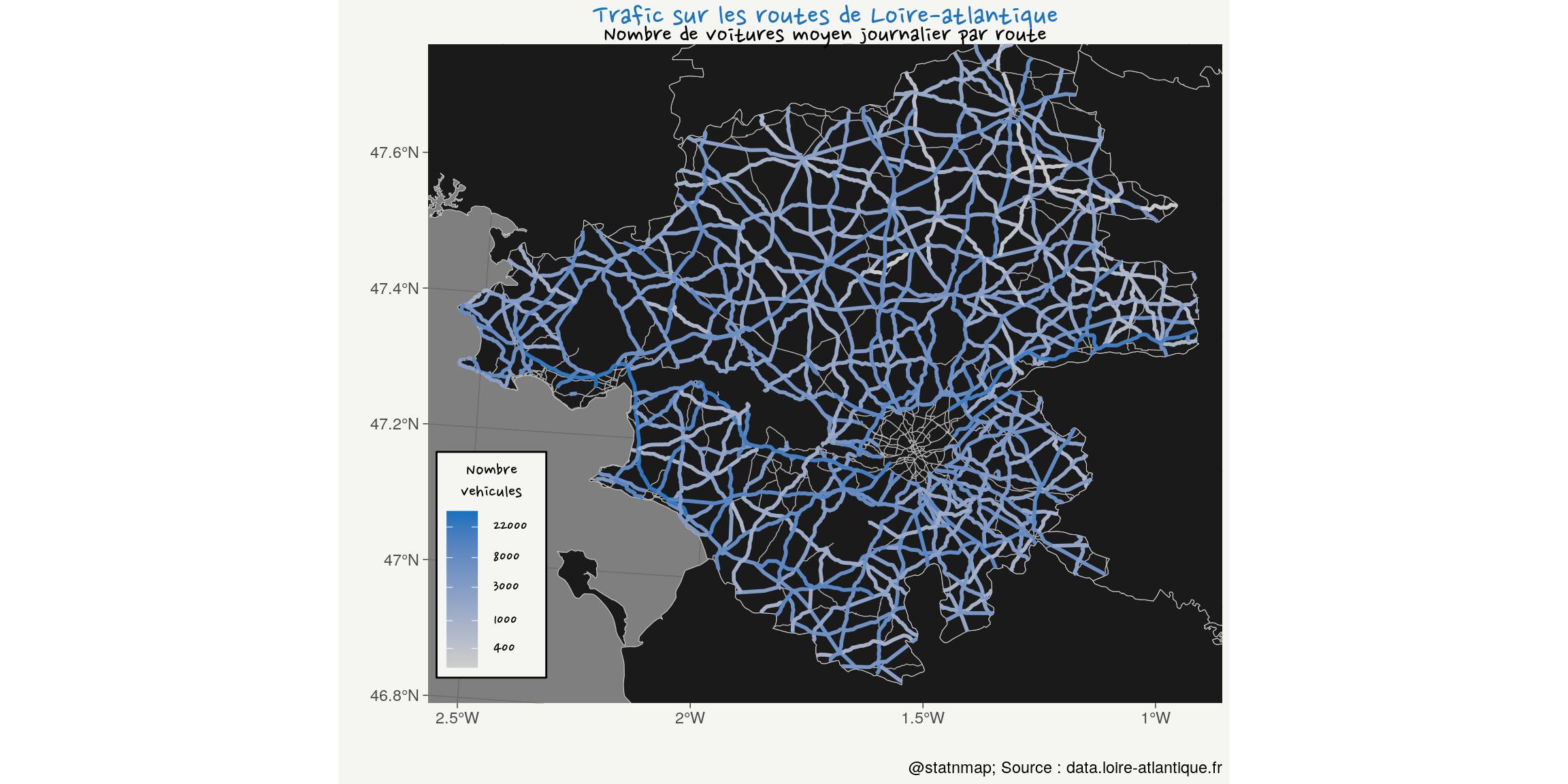
Lignes : Colorer des routes en fonction d’une variable numérique avec {ggplot2}

# Figure
ggplot() +
  geom_sf(data = LoireATl_L93, colour = "grey80", fill = "grey10", size = 0.2) +
  geom_sf(data = RoadsMergeTrafic_Dpt44_L93, colour = "grey70", size = 0.25) +
  geom_sf(data = filter(RoadsMergeTrafic_Dpt44_L93, !is.na(TV)),
          aes(colour = TV),
          # aes(alpha = -TV, size = TV), # No alpha with lines
          size = 1,
          show.legend = "line", inherit.aes = FALSE) +
  coord_sf(crs = st_crs(trafic_L93)) +
  xlim(st_bbox(trafic_L93)$xmin, st_bbox(trafic_L93)$xmax) +
  ylim(st_bbox(trafic_L93)$ymin, st_bbox(trafic_L93)$ymax) +
  scale_colour_gradient(
    low = "grey80", 
    high = my_blue,
    trans = "log", breaks = c(400, 1000, 3000, 8000, 22000)
  ) +
  labs(x = "", y = "", 
       title = "Trafic sur les routes de Loire-atlantique",
       subtitle = "Nombre de voitures moyen journalier par route",
       caption = "@statnmap; Source : data.loire-atlantique.fr",
       colour = "Nombre\nvehicules"
  ) +
  my_theme(
    legend.position = c(0.08, 0.21)
  )

Polygones : Fusions de polygones et zones tampons intérieures

Polygones en polygones.
Inspiré de mon post de blog Un halo teinté à l’intérieur d’un polygone avec leaflet et la librairie {sf}

# France union
France_union_L93 <- st_union(France_L93)
# _Negative buffer on France
France_dough <- st_buffer(France_union_L93, dist = -15000) %>% 
  st_difference(France_union_L93, .)

# Pays de la loire union
PaysLoire_union_L93 <- France_L93 %>% 
  filter(NOM_REG == "PAYS DE LA LOIRE") %>% 
  st_union()
# _Negative buffer on PdL
PdL_dough <- st_buffer(PaysLoire_union_L93, dist = -10000) %>% 
  st_difference(PaysLoire_union_L93, .)

# Loire-atlantique
LoireATl_small_L93 <- filter(LoireATl_L93, NOM_DEPT == "LOIRE-ATLANTIQUE")
# Negative buffer 1 on LA
LoireATl_dough1 <- st_buffer(LoireATl_small_L93, dist = -5000) %>% 
  st_difference(LoireATl_small_L93, .)
# Negative buffer 2 on LA
LoireATl_dough2 <- st_buffer(LoireATl_small_L93, dist = -15000) %>% 
  st_difference(st_buffer(LoireATl_small_L93, dist = -10000), .)
# Negative buffer 3 on LA
LoireATl_dough3 <- st_buffer(LoireATl_small_L93, dist = -25000) %>% 
  st_difference(st_buffer(LoireATl_small_L93, dist = -20000), .)

# Plot
ggplot() +
  # France
  geom_sf(data = France_union_L93, fill = "grey50", colour = "grey20", size = 2) +
  geom_sf(data = France_dough, fill = my_blue, colour = NA) +
  # PdL
  geom_sf(data = PaysLoire_union_L93, fill = "grey70", colour = "grey20", size = 1.5) +
  geom_sf(data = PdL_dough, fill = my_blue, colour = NA) +
  # LA
  geom_sf(data = LoireATl_small_L93, fill = "grey90", colour = "grey20", size = 1) +
  geom_sf(data = LoireATl_dough1, fill = my_blue, colour = NA) +
  geom_sf(data = LoireATl_dough2, fill = my_blue, colour = NA) +
  geom_sf(data = LoireATl_dough3, fill = my_blue, colour = NA) +
  labs(
    title = "Loire-atlantique department...",
    subtitle = "...in Pays de la Loire region, in France",
    caption = "@statnmap; Source : ign.fr"
  ) +
  my_theme()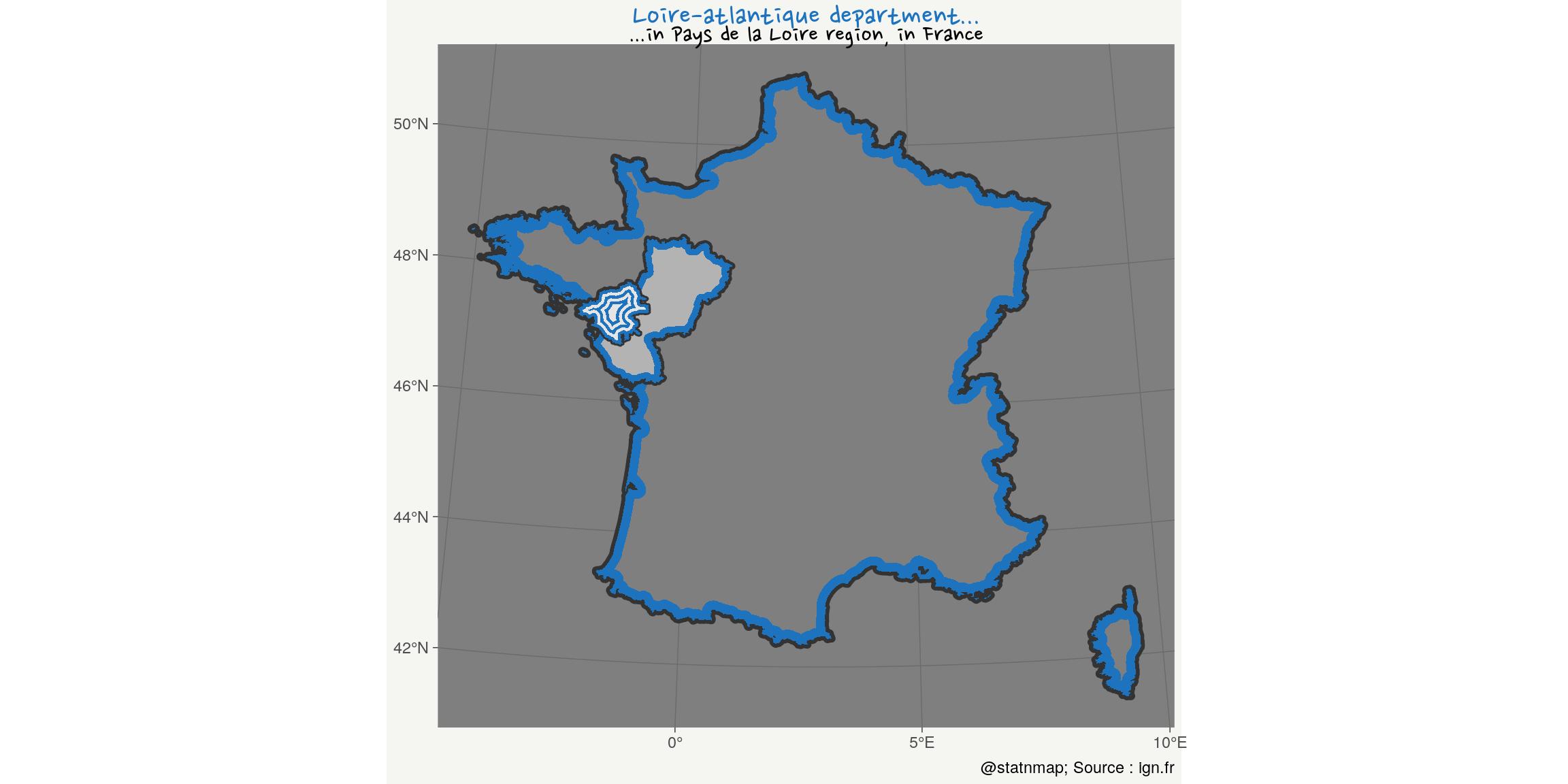

Hexagones : Dessiner des hexagones et transformer en données géographiques de polygones

La France c’est “L’Hexagone”. Regardons pourquoi !

# France in hex
fr_bbox <- st_bbox(France_L93 %>% filter(!grepl("CORSE", NOM_DEPT)))
fr_hex <- hexbin::hexcoords(
  dx = (fr_bbox$xmax - fr_bbox$xmin)/2 + 15000
) %>% 
  as_tibble() %>% 
  bind_rows(.[1,]) %>% 
  mutate(
    id = 1:n(),
    x = x + fr_bbox$xmin + 0.5 * (fr_bbox$xmax - fr_bbox$xmin) + 20000,
    y = y + fr_bbox$ymin + 0.5 * (fr_bbox$ymax - fr_bbox$ymin) - 30000
  ) %>% 
  st_as_sf(coords = c("x", "y"), crs = 2154) %>% 
  st_combine() %>% 
  st_cast("POLYGON")

# Corse in hex
c_bbox <- st_bbox(France_L93 %>% filter(grepl("CORSE", NOM_DEPT)))
c_hex <- hexbin::hexcoords(
  dx = (c_bbox$xmax - c_bbox$xmin)/2 + 20000,
  dy = (c_bbox$ymax - c_bbox$ymin)/3
) %>% 
  as_tibble() %>% 
  bind_rows(.[1,]) %>% 
  mutate(
    id = 1:n(),
    x = x + c_bbox$xmin + 0.5 * (c_bbox$xmax - c_bbox$xmin),
    y = y + c_bbox$ymin + 0.5 * (c_bbox$ymax - c_bbox$ymin)
    ) %>% 
  st_as_sf(coords = c("x", "y"), crs = 2154) %>% 
  st_combine() %>% 
  st_cast("POLYGON")

ggplot() +
  geom_sf(data = fr_hex, fill = NA, colour = my_blue, size = 2) +
    geom_sf(data = c_hex, fill = NA, colour = my_blue, size = 2) +
  geom_sf(data = France_union_L93, fill = "grey60",
          colour = "grey20", size = 1) +
    labs(
      title = "France = L'Hexagone (regulier)",
      subtitle = "La Corse aussi (presque)...",
      caption = "@statnmap; Source : ign.fr"
    ) +
  my_theme()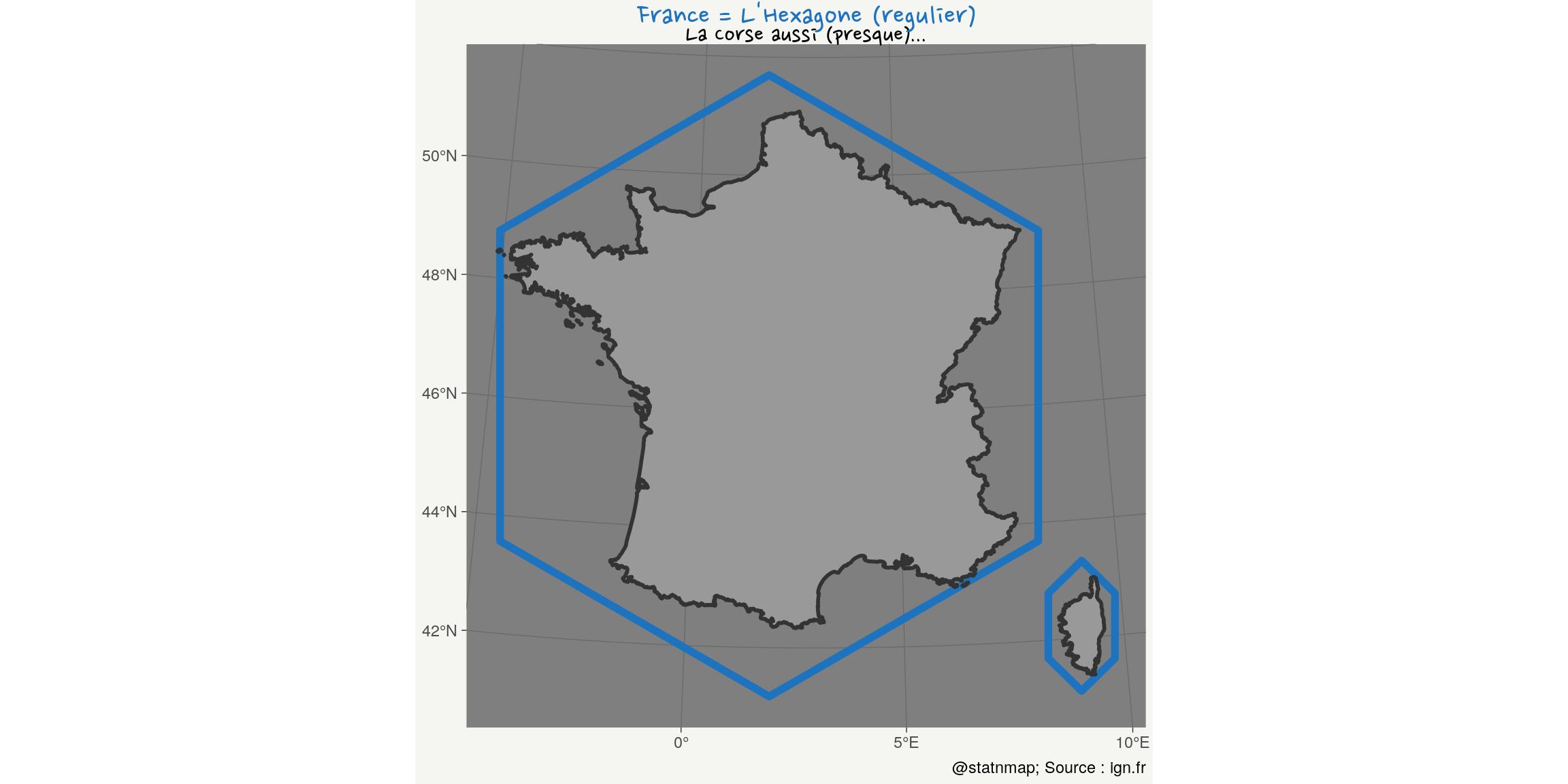

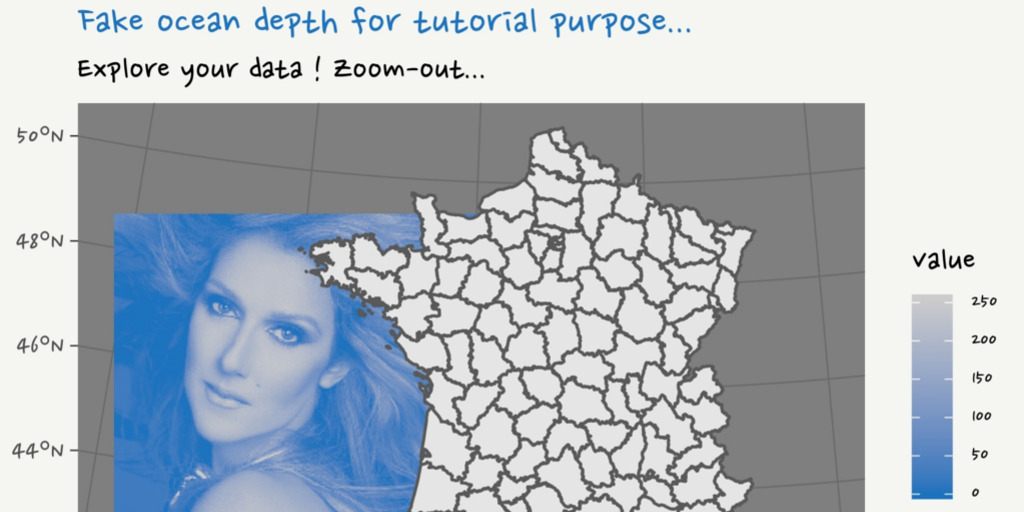
Raster : Les images sont des rasters qui s’ajoutent aux cartes

Les images sont des rasters. Si vous n’êtes pas convaincus, vous pouvez regarder mes articles dans la catégorie “geohacking”. Vous pouvez aussi regarder ma présentation à SatRday Paris 2019 : 2019-02 - Everything but maps with spatial tools - SatRday Paris (EN).

Un jour, j’ai donné un tutoriel sur QGIS à des étudiants en master à l’Université. Ils observaient une zone d’étude spécifique. Je leur ai demandé de charger un fichier raster bathymétrique pour qu’ils puissent en extraire la profondeur aux positions d’échantillonnage. Comme le projet était déjà zoomé sur la zone, ils n’ont pas remarqué que le fichier raster était en fait une image de Céline Dion…
L’objectif était de leur dire qu’ils devaient explorer leurs données et être sûrs de ce qu’ils manipulent avant de les utiliser pour toute analyse. J’espère qu’ils ont compris le message…
Comment reproduire ceci en utilisant R ?

# image: 1125*1500
xmin <- -300000; xmax <- 800000; ymin <- 6100000
r <- raster::raster(file.path(extraWD, "celine-dion.jpeg"),
                    crs = st_crs(France_L93)$proj4string)
extent(r) <- c(xmin, xmax, ymin,  ymin + ((xmax-xmin)*1125/1500))

ext <- c(xmin = 250000, xmax = 500000, ymin = 6400000, ymax = 6800000)
cropping_area <-  st_bbox(ext) %>% st_as_sfc()
r_cropped <- raster::crop(r, extent(ext))
France_cropped <- France_L93 %>% st_crop(cropping_area)

rasterVis::gplot(r_cropped, maxpixels = 750000) +
  geom_tile(aes(fill = value)) +
  geom_sf(data = France_cropped, inherit.aes = FALSE) +
  scale_fill_gradient(
    low = my_blue, 
    high = "grey80"
  ) +
  labs(
    title = "Fake ocean depth for tutorial purpose...",
    subtitle = "Explore your data !",
    caption = "@statnmap",
    x = NULL, y = NULL
  ) +
  coord_sf(expand = FALSE) +
  my_theme()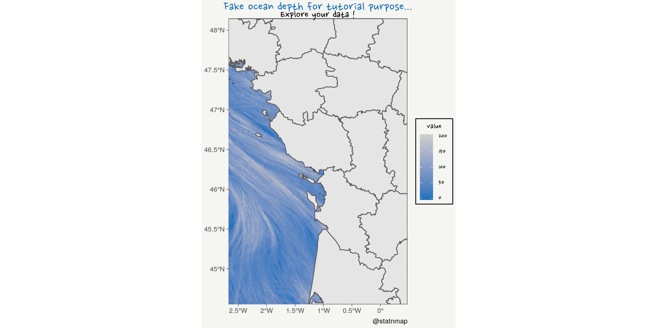

Zoom-out !

rasterVis::gplot(r, 100000) +
  geom_tile(aes(fill = value)) +
  geom_sf(data = France_L93, inherit.aes = FALSE) +
  scale_fill_gradient(
    low = my_blue, 
    high = "grey80"#,
    # trans = "log", breaks = c(400, 1000, 3000, 8000, 22000)
  ) +
  labs(
    title = "Fake ocean depth for tutorial purpose...",
    subtitle = "Explore your data ! Zoom-out...",
    caption = "@statnmap",
    x = NULL, y = NULL
  ) +
  my_theme()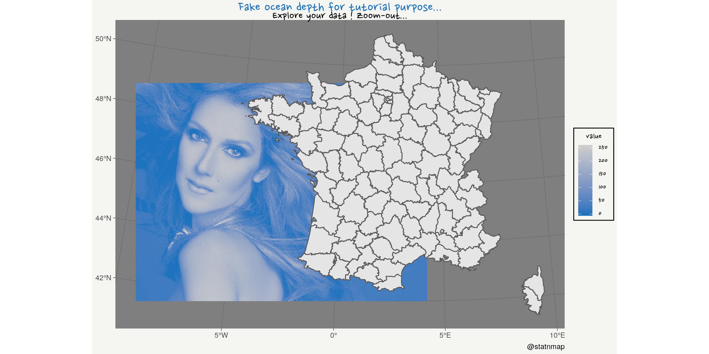

Bleu : Carte de probabilité de présence de poissons et encart avec {ggplot2}

Je suis avant tout un biologiste marin, à qui la couleur bleu fait penser à l’océan. Voyons si je peux ressortir les distributions prédites de juvéniles de soles estimées lors de mon doctorat…

Rochette, S., Rivot, E., Morin, J., Mackinson, S., Riou, P., Le Pape, O. (2010). Effect of nursery habitat degradation on flatfish population renewal. Application to Solea solea in the Eastern Channel (Western Europe). Journal of sea Research, Volume 64, p34-44. doi: 10.1016/j.seares.2009.08.003 , Open Access version : http://archimer.ifremer.fr/doc/00008/11921/.

# World map
countries <- rnaturalearth::ne_countries(returnclass = "sf", scale = "large")
# Europe
Europe <- countries %>% 
  filter(continent == "Europe")
# Proba presence solea
solea <- raster(file.path(extraWD,
                          "Raster_PresenceProbability_Predictions.tif"))

# Projet raster to L93
solea_l93 <- projectRaster(
  solea,
  crs = st_crs(France_L93)$proj4string)

# Window
g_window <- ggplot() +
  geom_sf(data = Europe, fill = "white") +
  geom_sf(data = st_bbox(solea_l93) %>% st_as_sfc(),
          colour = my_blue, fill = NA, size = 2) +
  coord_sf(xlim = c(-10, 20), ylim = c(40, 60),
           expand = FALSE) +
  theme_bw() +
  theme(
    panel.background = element_rect(
      fill = scales::alpha(my_blue, 0.5)),
    axis.text = element_blank(),
    axis.ticks = element_blank()
    )

# Solea img
img_solea <- magick::image_read(file.path(extraWD, "Solea.gif"))
g_solea <- magick::image_ggplot(img_solea)

# Plot
rasterVis::gplot(solea_l93, maxpixels = 1623075) +
  geom_tile(aes(fill = value)) +
  geom_sf(data = Europe, inherit.aes = FALSE,
          size = 0.1, fill = "white") +
  scale_fill_gradient(
    high = my_blue, 
    low = "grey80", na.value = NA,
    limits = c(0, NA)
  ) +
  labs(
    title = "Probability of presence of Young-of-the-year common sole",
    subtitle = "Eastern Channel",
    caption = "@statnmap",
    x = NULL, y = NULL,
    fill = "Probability"
  ) +
  coord_sf(crs = 2154, 
             xlim = bbox(solea_l93)[1,],
           ylim = bbox(solea_l93)[2,]) +
  my_theme() +
  annotation_custom(grob = ggplotGrob(g_window),
    xmin = 540000, xmax = 630000,
    ymin = 6882000, ymax = 6982000) +
  annotation_custom(grob = ggplotGrob(g_solea),
    xmin = 331500, xmax = 430000,
    ymin = 6982000, ymax = 7052000)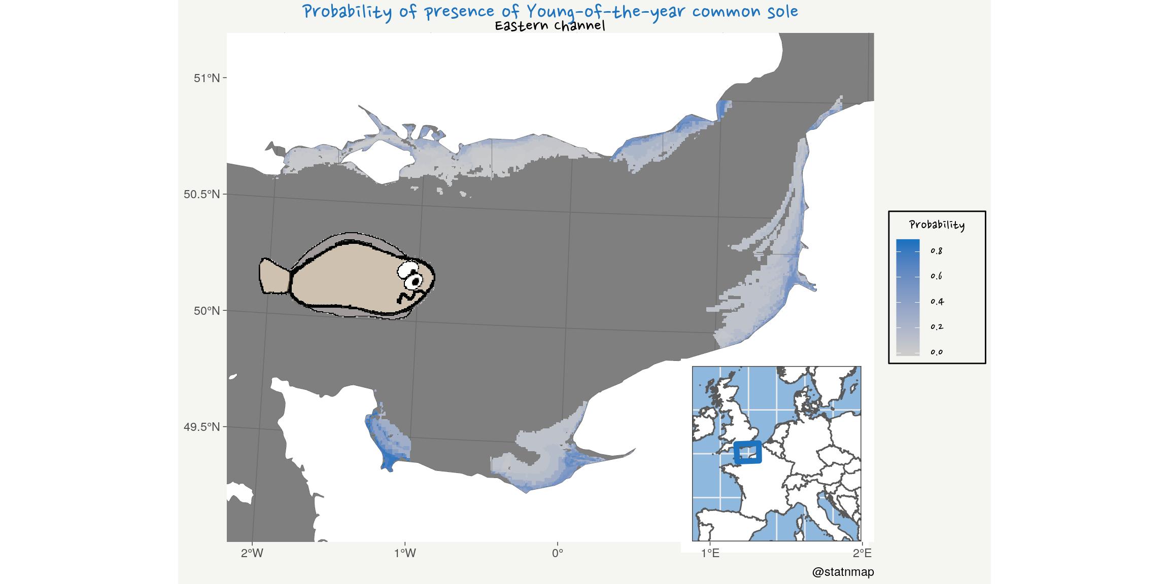

Rouge : Echantillonner un polygone selon une grille régulière hexagonale

Où peut-on boire un verre de vin rouge en France ? Utilisons la distribution des cafés/bars répertoriés dans OpenStreetMap et qui sont stockés par OpenDataSoft : Points d’Intérêt en France (depuis OpenStreetMap).
C’est l’occasion de tester le package de [@Tutuchan](https://twitter.com/Tutuchan), {fodr} pour télécharger les données depuis le portail de données libres français.

Pour jouer un peu avec les hexagones, nous allons transformer un nuage de points géographiques en grille hexagonale.
On peut supposer a priori que la distribution des bars et des cafés devrait suivre la distribution de la population. Dans le cas présent, cela est exagéré par la disponibilité des utilisateurs d’OpenStreetMap qui complètent l’information. Ainsi, l’absence apparente de bars/cafés dans certaines zones est plus probablement une conséquence de l’absence d’utilisateurs d’OSM, que de l’absence réelle. Parce qu’on sait bien qu’il y a des bars partout !

Ici, je télécharge séparément les données pour “bar” et “café”. Mais il y a quelques “cafés-bars” qui doivent ne pas être comptés deux fois. J’utilise la position géographique pour les fusionner avec {sf} et st_union.

file_bar <- file.path(extraWD, "bars.csv")
file_cafe <- file.path(extraWD, "cafes.csv")
if (!file.exists(file_bar) | !file.exists(file_cafe)) {
  # devtools::install_github("tutuchan/fodr")
  # portal <- fodr::fodr_portal("ods")
  poi <- fodr::fodr_dataset("ods", "points-dinterets-openstreetmap-en-france")
  
  # bars
  bars <- poi$get_records(refine = list(amenity = "bar"))
  
  bars_chr <- bars %>% 
    dplyr::select(-geo_shape)
  
  write_csv(bars_chr, file_bar)
  
  # cafes
  cafes <- poi$get_records(refine = list(amenity = "cafe"))
  
  cafes_chr <- cafes %>% 
    dplyr::select(-geo_shape)
  
  write_csv(cafes_chr, file_cafe)
} else {
  bars_chr <- read_csv(file_bar)
  cafes_chr <- read_csv(file_cafe)
}

bars_sf_l93 <- bars_chr %>% 
  st_as_sf(coords = c("lng", "lat"), crs = 4326) %>% 
  st_transform(crs = 2154)
cafes_sf_l93 <- cafes_chr %>% 
  st_as_sf(coords = c("lng", "lat"), crs = 4326) %>% 
  st_transform(crs = 2154)

cafes_bars_l93 <- rbind(bars_sf_l93, cafes_sf_l93 %>% dplyr::select(-other_tags))

# Too heavy. Rstudio breaks
# cafes_bars_union_l93 <- st_union(bars_sf_l93, cafes_sf_l93 %>% dplyr::select(-other_tags))

cafes_bars_combine_l93 <- st_union(cafes_bars_l93) %>% 
  st_cast("POINT") %>% 
  st_sf()

France_hex <- France_L93 %>% 
  st_make_grid(what = "polygons", square = FALSE,
               n = c(40, 20)) %>% 
  st_sf() %>% 
  mutate(id_hex = 1:n()) %>% 
  dplyr::select(id_hex, geometry)
# plot(France_hex)

# Join bars wth hex and count
bars_hex_l93 <- st_join(cafes_bars_combine_l93, France_hex)
bars_hex_count <- bars_hex_l93 %>% 
  st_drop_geometry() %>% 
  count(id_hex)

# Join hex with bars count
France_hex_bars <- France_hex %>% 
  left_join(bars_hex_count)

ggplot(France_hex_bars) +
  geom_sf(aes(fill = n), size = 0.1) +
    scale_fill_gradient(
    high = "#AD1128", #my_blue, 
    low = "grey80", na.value = NA,
    trans = "log", 
    breaks = c(0, 8, 50, 400)
  ) +
  labs(
    title = "Number of cafes/bars in France",
    subtitle = "From OpenStreetMap data. Yes, this is (almost) the map of the population...",
    caption = "@statnmap - source: public.opendatasoft.com",
    x = NULL, y = NULL,
    fill = "Number"
  ) +
  coord_sf(crs = 2154) +
  my_theme()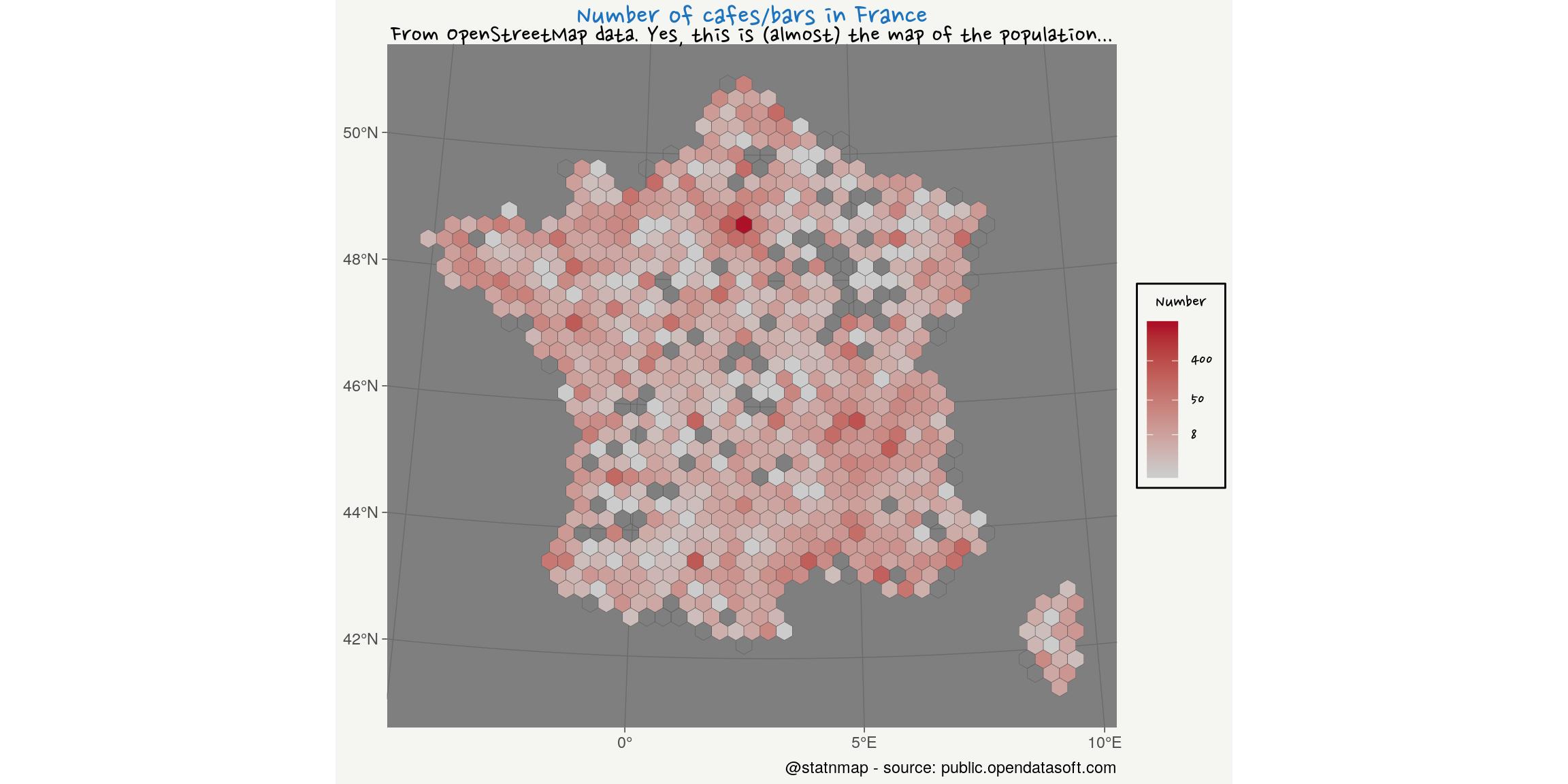

Maintenant que vous avez vu différentes façons de créer des cartes dans R avec {ggplot2}, vous pouvez aller voir les autres articles du challenge :

Comme toujours, le code et les données de cet article est disponible sur https://github.com/statnmap/blog_tips

# Biblio with {chameleon}
tmp_biblio <- tempdir()
attachment::att_from_rmd("2019-11-08-30daymapchallenge-building-maps-1.Rmd", inside_rmd = TRUE) %>% 
  chameleon::create_biblio_file(
    out.dir = tmp_biblio, to = "html", edit = FALSE)
htmltools::includeMarkdown(file.path(tmp_biblio, "bibliography.html"))

List of dependencies

dplyr (Wickham, François, et al. (2020))
sf (Pebesma (2020))
raster (Hijmans (2020))
ggplot2 (Wickham, Chang, et al. (2020))
readr (Wickham, Hester, and Francois (2018))
tmap (Tennekes (2020))
extrafont (Winston Chang (2014))
attachment (Guyader and Rochette (2020))
chameleon (Rochette (2020))
htmltools (RStudio and Inc. (2019))

References

Guyader, Vincent, and Sébastien Rochette. 2020. Attachment: Deal with Dependencies. https://github.com/Thinkr-open/attachment.

Hijmans, Robert J. 2020. Raster: Geographic Data Analysis and Modeling. https://CRAN.R-project.org/package=raster.

Pebesma, Edzer. 2020. Sf: Simple Features for R. https://CRAN.R-project.org/package=sf.

Rochette, Sébastien. 2020. Chameleon: Build and Highlight Package Documentation with Customized Templates. https://github.com/Thinkr-open/chameleon.

RStudio, and Inc. 2019. Htmltools: Tools for Html. https://CRAN.R-project.org/package=htmltools.

Tennekes, Martijn. 2020. Tmap: Thematic Maps. https://CRAN.R-project.org/package=tmap.

Wickham, Hadley, Winston Chang, Lionel Henry, Thomas Lin Pedersen, Kohske Takahashi, Claus Wilke, Kara Woo, Hiroaki Yutani, and Dewey Dunnington. 2020. Ggplot2: Create Elegant Data Visualisations Using the Grammar of Graphics. https://CRAN.R-project.org/package=ggplot2.

Wickham, Hadley, Romain François, Lionel Henry, and Kirill Müller. 2020. Dplyr: A Grammar of Data Manipulation. https://CRAN.R-project.org/package=dplyr.

Wickham, Hadley, Jim Hester, and Romain Francois. 2018. Readr: Read Rectangular Text Data. https://CRAN.R-project.org/package=readr.

Winston Chang. 2014. Extrafont: Tools for Using Fonts. https://CRAN.R-project.org/package=extrafont.

Citation :

Merci de citer ce travail avec :
Rochette Sébastien. (2019, nov.. 08). "#30DayMapChallenge: 30 jours de création de cartes (1) - ggplot2". Retrieved from https://statnmap.com/fr/2019-11-08-30daymapchallenge-creer-cartes-1/.

Citation BibTex :

@misc{Roche2019#30Da,
    author = {Rochette Sébastien},
    title = {#30DayMapChallenge: 30 jours de création de cartes (1) - ggplot2},
    url = {https://statnmap.com/fr/2019-11-08-30daymapchallenge-creer-cartes-1/},
    year = {2019}
  }