Suivre une trajectoire de particule sur un raster avec {rayshader}

· 2365 mots. · 12 minutes de lecture.

spatial · r-scripts · geohacking

rstatsFR · rayshader · raster · trajectoires · video

{rayshader} est un package fantastique pour la cartographie 3D, mais il vient avec les limitations de {rgl}. J’ai toujours trouvé dommage de ne pas pouvoir me balader dans toutes les directions sur mes objets 3D. Dans ce billet de blog, je vais vous montrer une astuce pour simuler la trajectoire des particules en 3 dimensions comme dans un jeu vidéo “à la première personne”.

Les fonctions présentées dans cet article sont disponibles dans le package {maps2ray} sur mon Github: https://github.com/statnmap/maps2ray

Quelques années plus tôt…..

Il y a quelques années, je modélisais la dispersion des larves de poissons plats dans la Manche orientale pour ma thèse de doctorat (Lien vers la thèse au bas de mon CV). A cette époque, je rêvais que j’aurais le temps de créer une petite vidéo qui suivrait une larve pendant son long voyage vers la côte, pour ensuite devenir un jeune poisson plat…. Je n’ai jamais trouvé le temps de faire ça. La seule animation que j’ai pu faire était celle qui suit. Les changements de symbole des particules sont selon le stade de développement des larves. À un moment donné, elles peuvent s’installer au-dessus d’une nourricerie, si elles en atteignent une…

Traduit avec www.DeepL.com/Translator

Figure 1: Solea solea larval dispersal

Maintenant, avec {rayshader}, mes rêves peuvent devenir réalité !

Packages

# devtools::install_github("tylermorganwall/rayshader")
# remotes::install_github("statnmap/mesh2ray")
library(rayshader)
library(sf)
library(raster)
library(rasterVis)
library(ggplot2)
library(dplyr)
library(rgl)

Récupérer une carte d’altitude

Cette carte est une carte d’altitude de la Loire-atlantique, en France, récupérée sur le site de l’IGN.

# extraWD <- "." # Uncomment for the script to work
if (!file.exists(file.path(extraWD, "Alti_mosaic_L93.tif"))) {
  # Download data
  githubURL <- "https://github.com/statnmap/blog_tips/raw/master/2019-10-06-follow-moving-particle-trajectory-on-raster-with-rayshader/Alti_mosaic_L93.tif"
  download.file(githubURL, destfile =  file.path(extraWD, "Alti_mosaic_L93.tif"))
}
  
altitude <- raster(file.path(extraWD, "Alti_mosaic_L93.tif")) # %>% 
  # aggregate(fact = 2)
plot(altitude)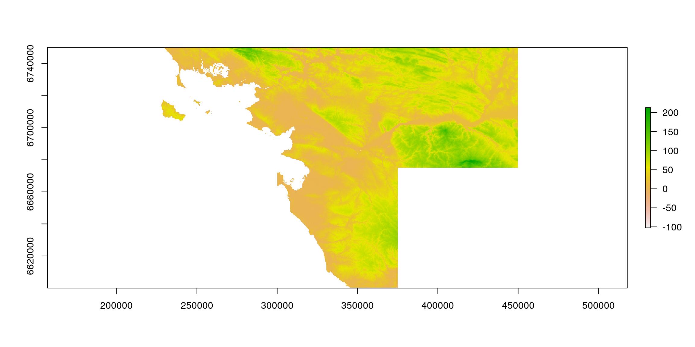

Figure 2: Loire-atlantique Altitude

Créer une trajectoire en tant qu’objet spatial {sf}

Nous créons d’abord une ligne droite que nous pouvons échantillonner en point espacés de manière régulière.

line_mat <- matrix(c(250000, 450000, 6720000, 6720000), ncol = 2)
line_traject <- st_linestring(x = line_mat)
point_traject <- st_sample(line_traject, size = 50, type = "regular") %>% 
  st_set_crs(2154) %>% 
  st_sf()

# Plot
gplot(altitude) +
  geom_tile(aes(fill = value)) +
  geom_sf(data = point_traject, colour = "white", inherit.aes = FALSE) +
  scale_fill_viridis_c()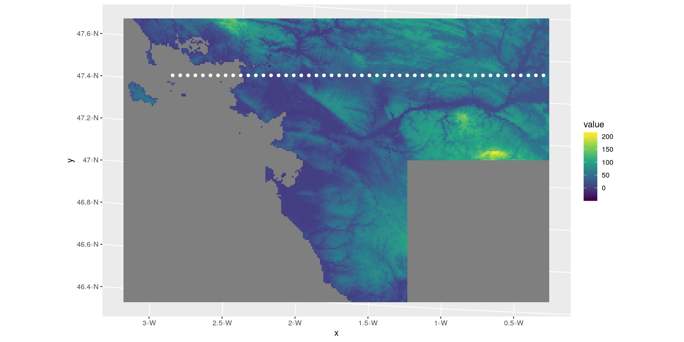

Figure 3: Simple trajectory with {sf}

Créer une fonction pour transformer un objet {sf} prêt pour {rayshader}

Ce n’est pas un secret, j’aime bien jouer avec {rayshader}. D’autres de mes articles montrent mes expériences avec {rayshader}. J’aime aussi jouer avec les objets géographiques. Pour cela, le package {sf} permet un bon début.
C’est pourquoi, dans mon exposé intitulé “Tout sauf des cartes avec des outils spatiaux” à SatRday Paris, j’ai présenté quelques visualisations 3D superposées à des objets spatiaux {sf}. Je ne pense pas avoir partagé le scripts de cette présentation. Alors le voici.
Vous trouverez ci-dessous une fonction qui modifie les objets {sf} à superposer sur un objet {raster} en utilisant {rayshader} : sf_proj_as_ray(). Celui-ci recalcule les positions dans le futur système de coordonnées de référence de votre raster transformé pour le rayshading.
Cette fonction est dans le package {maps2ray} sur mon Github: https://github.com/statnmap/maps2ray

#' Modify sf data to plot over rayshader
#'
#' @param r original raster used in rayshader
#' @param sf sf object to add on plot (with or without z column)
#' @param z_pos z-position of the sf on the 3d map if not in dataset
#' @param zscale if z-column existed in the dataset
#' @param as_sf Logical. Return sf object or not
#' @param groups Logical. Whether to group coordinates in blocks according to original structure. 
#' @param crop Whether to crop sf object to extent of raster
#' 
#' @export
sf_proj_as_ray <- function(r, sf, z_pos = 1, zscale = 10, as_sf = TRUE, groups = TRUE, crop = TRUE) {
  
  # Crop to extent of raster
  if (isTRUE(crop)) {
    sf <- st_crop(sf, st_bbox(r))
  }
  
  if (!is.null(sf$z)) {
    sf <- sf %>% 
      mutate(
        L2 = 1:n(),
        Z_ray = z / zscale
      )
  } else {
    sf <- sf %>% 
      mutate(
        L2 = 1:n(),
        Z_ray = z_pos / zscale
      )
  }
  
  coords <- sf %>% 
    st_coordinates() %>% 
    as.data.frame() %>% 
    as_tibble() %>% 
    mutate(
      X_ray = (X - xmin(r)) / xres(r),
      # Y_ray = -1*(Y - ymin(r)) / yres(r)
      Y_ray = 1*(Y - ymin(r)) / yres(r)
    )
  
  if (!"L1" %in% names(coords)) {
    coords <- coords %>% 
      mutate(L1 = 1,
             L2 = 1:n()
      )
  } else if (!"L2" %in% names(coords)) {
    coords <- coords %>% 
      group_by(L1) %>% 
      mutate(L2 = L1,
             L1b = 1:n()) %>% 
      ungroup() %>% 
      mutate(L1 = L1b) %>% 
      select(-L1b)
  }
  
  if (isTRUE(as_sf)) {
    coords_sf <- coords %>% 
      select(-X, -Y) %>% 
      st_as_sf(coords = c("X_ray", "Y_ray")) %>% 
      group_by(L1, L2) %>% 
      summarise(do_union = FALSE) %>% 
      left_join(as.data.frame(sf) %>% select(-geometry))
    
    if (all(st_is(sf, c("POLYGON", "MULTIPOLYGON")))) {
      coords_sf <- coords_sf %>% 
        st_cast("POLYGON")
    } else  if (all(st_is(sf, c("LINESTRING", "MULTILINESTRING")))) {
      coords_sf <- coords_sf %>% 
        st_cast("LINESTRING")
    }else if (all(st_is(sf, c("POINT", "MULTIPOINT")))) {
      coords_sf <- coords_sf %>% 
        st_cast("POINT")
    }
  } 
  if (isTRUE(groups)) {
    coords_grp <- coords %>% 
      mutate(Y_ray = -1 * Y_ray) %>% 
      left_join(st_drop_geometry(sf)) %>% 
      group_by(L1, L2) %>% 
      tidyr::nest(coords = c(X_ray, Z_ray, Y_ray))
  }
  
  if (isTRUE(as_sf) & isTRUE(groups)) {
    res <- list(sf = coords_sf, coords = coords_grp)
  } else if (isTRUE(as_sf) & !isTRUE(groups)) {
    res <- list(sf = coords_sf, coords = coords)
  } else if (isTRUE(as_sf) & !isTRUE(groups)) {
    res <- list(coords = coords_grp)
  } else {
    res <- list(coords = coords)
  }
  return(res)
}

Montrer les points sur l’image raster en rayshader

Maintenant, vous pouvez tracer les sorties de la fonction.

Calculer les coordonnées de l’objet {sf} dans le futur système de coordonnées de {rayshader} en utilisant sf_proj_as_ray()``. + Définir lazscale <- 10` pour tous les objets {rayshader}.

zscale <- 5
points_ray <- sf_proj_as_ray(r = altitude, sf = point_traject,
                             z_pos = maxValue(altitude) + 10,
                             zscale = zscale)

Créer le raster de terrain pour {rayshader} qui sera utilisé pour les images 2D et 3D.

# Transform raster as matrix
datamat <- t(as.matrix(altitude))
# Rayshade raster
ambmat <- ambient_shade(datamat, zscale = zscale)
raymat <- ray_shade(datamat, zscale = zscale, lambert = TRUE)

# Create ray_image
ray_image <- datamat %>%
  sphere_shade(texture = "imhof4") %>%
  add_shadow(raymat, max_darken = 0.5) %>%
  add_shadow(ambmat, max_darken = 0.5)

Créer l’image {rayshader} en 2D et ajouter des points avec le nouveau système de coordonnées de référence : sf dans la sortie de sf_proj_as_ray().
- Le point rouge est un objectif pour les paragraphes suivants

# plot rayshader in 2D
plot_map(ray_image)
plot(points_ray$sf, col = "blue", pch = 20, add = TRUE, reset = FALSE)
plot(points_ray$sf[10,], col = "red", pch = 20, cex = 2, add = TRUE, reset = FALSE)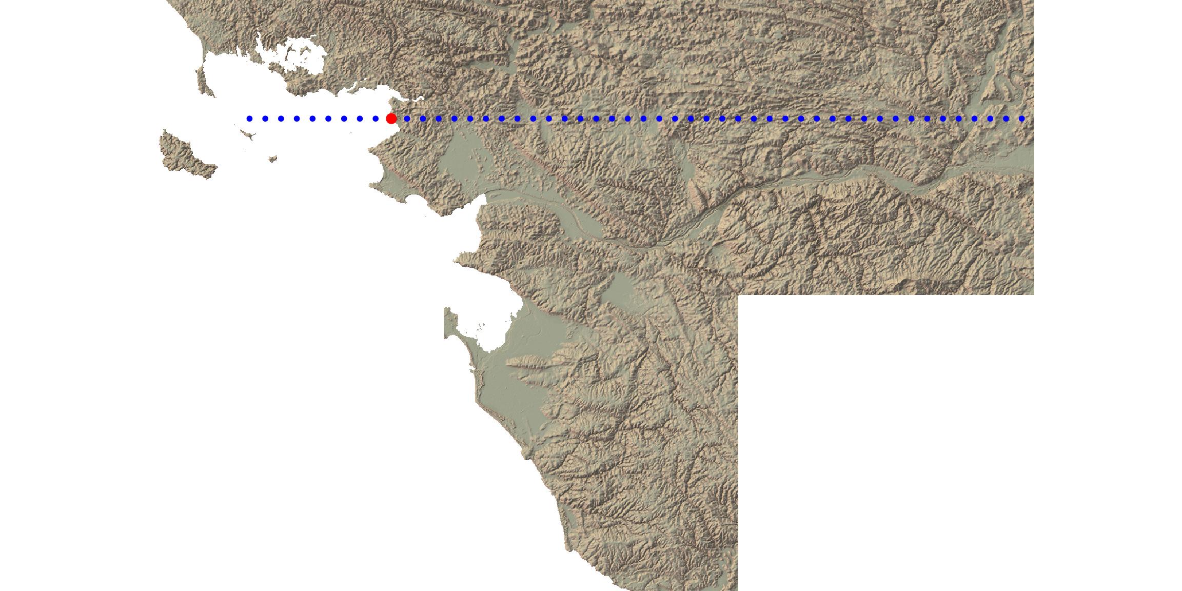

Figure 4: Trajectory over {rayshader} in 2D

Tracer l’image {rayshader} en 3D et superposer les points avec le nouveau système de coordonnées de référence : coords dans la sortie de sf_proj_as_ray().

ray_image %>% 
  plot_3d(
    datamat,
    zscale = zscale, windowsize = c(500, 500),
    soliddepth = -max(datamat, na.rm = TRUE)/zscale,
    water = TRUE, wateralpha = 0,
    theta = 15, phi = 40,
    zoom = 0.6, 
    fov = 60)

spheres3d(
  bind_rows(points_ray$coords$coords),
  col = "blue", add = TRUE, radius = 10,
  alpha = 1)

i <- 10
spheres3d(
  points_ray$coords$coords[[i]],
  col = "red", add = TRUE, radius = 20,
  alpha = 1)

rgl::snapshot3d(file.path(extraWD, "ray3dtotal.png"))
rgl::rgl.close()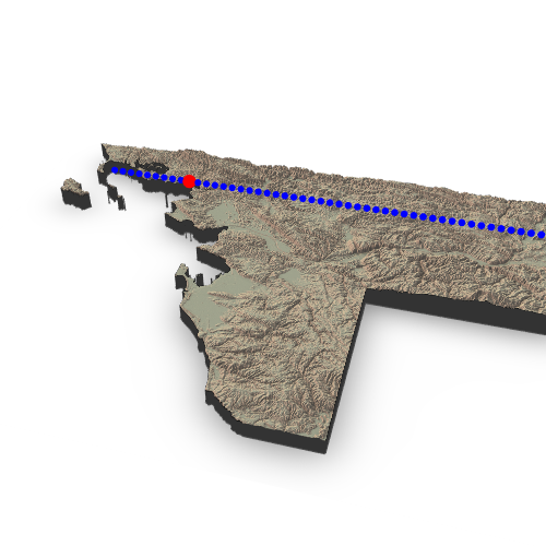

Figure 5: Trajectory over {rayshader} in 3D

Montrer une zone recadrée

Le raster est déjà rayshadé. Si je veux zoomer sur une zone spécifique, je n’ai pas envie de recalculer l’ombrage. J’ai donc exploré le système de référence pour recadrer les matrices et recalculer la position des points sur une partie plus petite du raster.
Pour ça, je me concentre sur un point de la trajectoire (le rouge des images au-dessus) et crée une fenêtre plus petite autour de ce point.

Nous pouvons vérifier que le recadrage est correct en 2D

# plot rayshader in 2D
dim(ray_image)
dim(datamat)
# Need a matrix without zero for render_label
data1 <- datamat
data1[is.na(data1)] <- 0

# Point as reference
i <- 10
position <- points_ray$coords$coords[[i]]
window <- 100
# Create a window around point
bounds <- tibble(
    Xmin = max(round(position)[1] - window, 0), # X
    Xmax = min(round(position)[1] + window, dim(datamat)[1]),
    Ymin_pos = max(round(position)[3] - window, -dim(datamat)[2]), # Y
    Ymax_pos = min(round(position)[3] + window, 0),
    Ymin_row = dim(datamat)[2] + Ymin_pos + 1,
    Ymax_row = dim(datamat)[2] + Ymax_pos + 1
)

# Height of the block (min - 1/5 of total height) to correct z
# soliddepth <- min(datamat, na.rm = TRUE))/zscale)
one_5 <- (max(datamat, na.rm = TRUE) - min(datamat, na.rm = TRUE))/5
soliddepth <- (min(datamat, na.rm = TRUE) - one_5)/zscale
  
# Calculate new position of the point on the cropped raster
position_bounds <- position %>% 
  mutate(
    X_ray = X_ray - bounds$Xmin + 1,
    Y_2d = Y_ray - bounds$Ymin_pos + 1,
    Y_ray = -1 * (Y_ray - bounds$Ymin_pos + 1),
    Z_ray = Z_ray
  )

# Verify cropped area and point position
plot_map(ray_image[bounds$Ymin_row:bounds$Ymax_row,bounds$Xmin:bounds$Xmax,])
points(position_bounds[,c("X_ray", "Y_2d")], col = "red", pch = 20, cex = 2)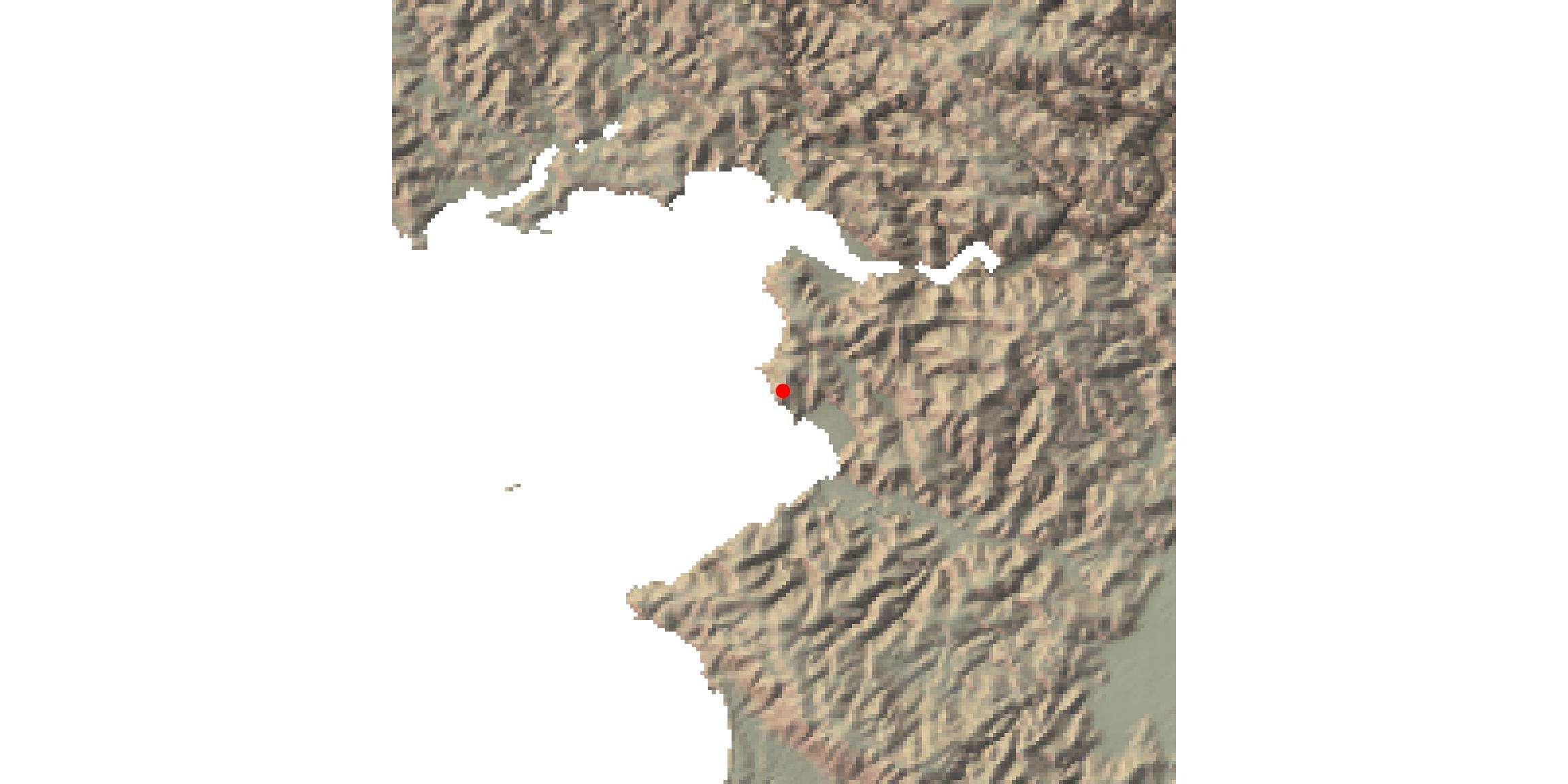

Figure 6: Verify cropping area in {rayshader} 2D

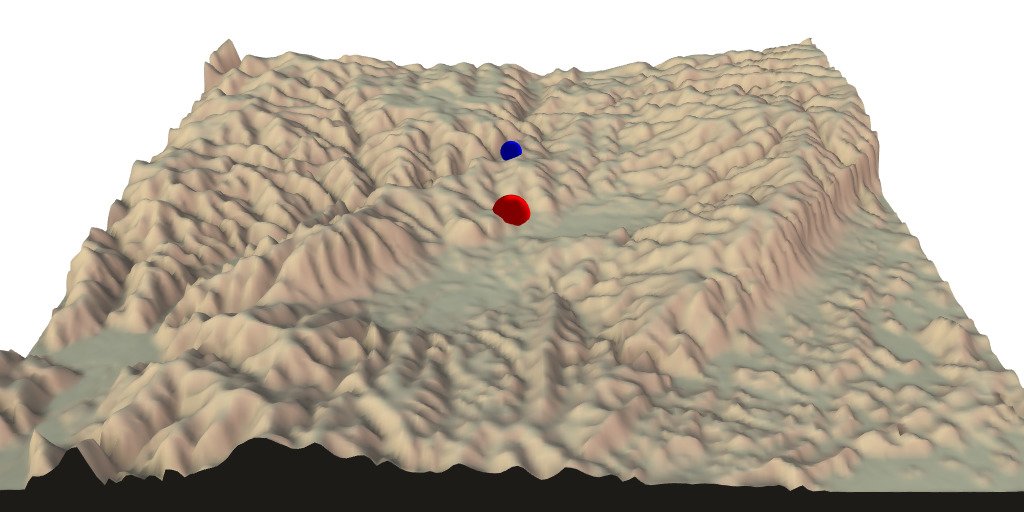
Puis en 3D

ray_image[bounds$Ymin_row:bounds$Ymax_row,bounds$Xmin:bounds$Xmax,] %>% 
  plot_3d(
    datamat[bounds$Xmin:bounds$Xmax, bounds$Ymin_row:bounds$Ymax_row],
    zscale = zscale, windowsize = c(500, 500),
    soliddepth = soliddepth,
    water = TRUE, wateralpha = 0,
    theta = -90, phi = 30, 
    zoom = 0.4, 
    fov = 80)

render_label(
  data1[bounds$Xmin:bounds$Xmax, bounds$Ymin_pos:bounds$Ymax_pos],
  x = pull(position_bounds[1, "X_ray"]),
  y = -pull(position_bounds[1, "Y_ray"]),
  z = 200,
  zscale = zscale,
  text = "Here",
  color = "red"
)

spheres3d(position_bounds[,c("X_ray", "Z_ray", "Y_ray")],
          color = "red", add = TRUE, lwd = 5, radius = 5,
          alpha = 1)

rgl::snapshot3d(file.path(extraWD, "ray3dcrop.png"))
rgl::rgl.close()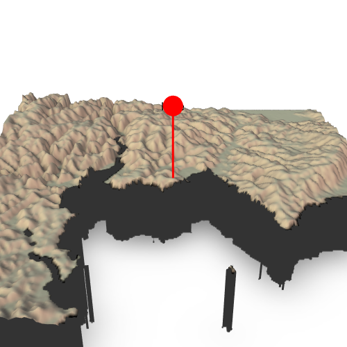

Figure 7: Trajectory over {rayshader} in 3D

Et si on faisait un film maintenant ?

Je peux créer les scènes autour de chaque point de la trajectoire et suivre une sphère sur la scène dans un gif.

Mettons tous les scripts ci-dessus ensemble dans une fonction

Cette fonction est dans le package {maps2ray} sur mon Github: https://github.com/statnmap/maps2ray

#' Create a cropped scene
#'
#' @param datamat Original raster transformed as matrix with t(as.matrix(raster))
#' @param ray_image Rayshaded image created with sphere_shade, add_shadow, ...
#' @param position dataframe of point coordinates in the {rayshader} system
#' as created using sf_proj_as_ray()
#' @param position_next dataframe of another point coordinates in the {rayshader} 
#'system as created using sf_proj_as_ray()
#' @param window size of the square window in pixels around the position
#' @param zscale Ratio between Z and x/y. Adjust the zscale down to exaggerate
#' elevation features. Better to use the same for the entire workflow.
#' @param zoom Zoom factor. Reduce to zoom in.
#' @param windowsize Size of the rgl window
render_cropped_scene <- function(ray_image, datamat, position,
                                 position_next,
                                 window = 100,
                                 zscale = 5, zoom = 0.4,
                                 windowsize = c(500, 500)) {
  # Create a window around point
  bounds <- tibble(
    Xmin = max(round(position)[1] - window, 0), # X
    Xmax = min(round(position)[1] + window, dim(datamat)[1]),
    Ymin_pos = max(round(position)[3] - window, -dim(datamat)[2]), # Y
    Ymax_pos = min(round(position)[3] + window, 0),
    Ymin_row = dim(datamat)[2] + Ymin_pos + 1,
    Ymax_row = dim(datamat)[2] + Ymax_pos + 1
  )

  # Height of the block (min - 1/5 of total height) to correct z
  # soliddepth <- min(datamat, na.rm = TRUE))/zscale)
  one_5 <- (max(datamat, na.rm = TRUE) - min(datamat, na.rm = TRUE))/5
  soliddepth <- (min(datamat, na.rm = TRUE) - one_5)/zscale
  
  # Calculate new position of the point on the cropped raster
  position_bounds <- position %>% 
    mutate(
      X_ray = X_ray - bounds$Xmin + 1,
      Y_2d = Y_ray - bounds$Ymin_pos + 1,
      Y_ray = -1 * (Y_ray - bounds$Ymin_pos + 1),
      Z_ray = Z_ray #/zscale
    )

  # Plot cropped 3D output
  ray_image[bounds$Ymin_row:bounds$Ymax_row,bounds$Xmin:bounds$Xmax,] %>% 
    plot_3d(
      datamat[bounds$Xmin:bounds$Xmax, bounds$Ymin_row:bounds$Ymax_row],
      zscale = zscale, windowsize = windowsize,
      # soliddepth = -min(datamat, na.rm = TRUE)/zscale,
      soliddepth = soliddepth,
      water = TRUE, wateralpha = 0,
      theta = -90, phi = 30, 
      zoom = zoom, 
      fov = 80)
  
  # Add point at position
  spheres3d(position_bounds[,c("X_ray", "Z_ray", "Y_ray")],
            color = "red", add = TRUE, lwd = 5, radius = 5,
            alpha = 1)

  if (!missing(position_next)) {
    position_next_bounds <- position_next %>% 
      mutate(
        X_ray = X_ray - bounds$Xmin + 1,
        Y_2d = Y_ray - bounds$Ymin_pos + 1,
        Y_ray = -1 * (Y_ray - bounds$Ymin_pos + 1),
        Z_ray = Z_ray
      )
    
    # Add point at position
    spheres3d(position_next_bounds[,c("X_ray", "Z_ray", "Y_ray")],
              color = "blue", add = TRUE, lwd = 5, radius = 3,
              alpha = 1)
  }
}

Créer un film en utilisant toutes les positions des points sur la trajectoire

path_gif <- file.path(extraWD, "film_follow_trajectory.gif")
if (!file.exists(path_gif)) {
  
  # Number of frame = Number of points
  n_frames <- length(points_ray$coords$coords)
  savedir <- file.path(extraWD, "film_follow_trajectory")
  if (!dir.exists(savedir)) {
    dir.create(savedir, showWarnings = FALSE)
  }
  img_frames <- file.path(
    savedir,
    paste0("film_", formatC(seq_len(n_frames), width = 3, flag = "0"), ".png")
  )
  
  # create all frames
  for (i in seq_len(n_frames)) {
    # i <- 20
    position <- points_ray$coords$coords[[i]]
    if (i < n_frames) {
      position_next <- points_ray$coords$coords[[i + 1]]
      render_cropped_scene(ray_image, datamat, position,
                           position_next)
    } else {
      # Last one
      render_cropped_scene(ray_image, datamat, position)
    }
    # Save img
    rgl::snapshot3d(img_frames[i])
    rgl::clear3d()
  }
  rgl::rgl.close()
  
  # Create gif
  magick::image_write_gif(magick::image_read(img_frames), 
                          path = path_gif, 
                          delay = 6/n_frames)
}

Figure 8: Film of trajectory over {rayshader} in 3D

Ajoutez les points avec des altitudes réelles

Extraire les altitudes aux positions des points pour mettre dans le film
Recalculer les positions avec le système de coordonnées de référence {rayshader}.
Construire le film !

# Extract z
point_traject_z <- point_traject %>% 
  st_cast("POINT") %>% 
  mutate(z = raster::extract(altitude, point_traject %>% st_cast("POINT")),
         z = ifelse(is.na(z), 4, z + 1))

points_ray_z <- sf_proj_as_ray(r = altitude, sf = point_traject_z,
                             zscale = zscale)

# Create film
path_gif_alt <- file.path(extraWD, "film_follow_trajectory_altitude.gif")
if (!file.exists(path_gif_alt)) {
  
  # Number of frame = Number of points
  n_frames <- length(points_ray_z$coords$coords)
  savedir <- file.path(extraWD, "film_follow_trajectory_altitude")
  if (!dir.exists(savedir)) {
    dir.create(savedir, showWarnings = FALSE)
  }
  img_frames <- file.path(
    savedir,
    paste0("film_", formatC(seq_len(n_frames), width = 3, flag = "0"), ".png")
  )
  
  # create all frames
  for (i in seq_len(n_frames)) {
    # i <- 20
    position <- points_ray_z$coords$coords[[i]]
    if (i < n_frames) {
      position_next <- points_ray_z$coords$coords[[i + 1]]
      render_cropped_scene(ray_image, datamat, position,
                           position_next)
    } else {
      # Last one
      render_cropped_scene(ray_image, datamat, position)
    }
    # Save img
    rgl::snapshot3d(img_frames[i])
    rgl::clear3d()
  }
  rgl::rgl.close()
  
  # Create gif
  magick::image_write_gif(magick::image_read(img_frames), 
                          path = path_gif_alt, 
                          delay = 6/n_frames)
}

Figure 9: Film of trajectory over {rayshader} in 3D

Allez plus loin

Retrouvez le script de ce post de blog sur mon github : https://github.com/statnmap/blog_tips
Les fonctions présentées dans cet article sont disponibles dans le package {maps2ray} sur mon Github: https://github.com/statnmap/maps2ray

Jouer avec {rayshader} : suivre le guide.
Suivez mon introduction à la cartographie en utilisant le package {sf}
Découvrez mes autres explorations de {rayshader}
Apprendre la cartographie avec R directement avec moi

Citation :

Merci de citer ce travail avec :
Rochette Sébastien. (2019, oct.. 06). "Suivre une trajectoire de particule sur un raster avec {rayshader}". Retrieved from https://statnmap.com/fr/2019-10-06-suivre-trajectoire-particule-sur-raster-avec-rayshader/.

Citation BibTex :

@misc{Roche2019Suivr,
    author = {Rochette Sébastien},
    title = {Suivre une trajectoire de particule sur un raster avec {rayshader}},
    url = {https://statnmap.com/fr/2019-10-06-suivre-trajectoire-particule-sur-raster-avec-rayshader/},
    year = {2019}
  }